Section 6.9 DRRHO Risk Minimization
As a last application of compositional optimization, we consider an emerging problems in AI. With the success of large foundation models, numerous companies and research groups have entered the race to develop state-of-the-art models. While the data and code are often proprietary, the resulting models are sometimes released publicly, such as the CLIP models from OpenAI. How can we leverage these open-weight models? We discuss three commonly used strategies and then present an emerging paradigm.
Using the Model As-Is
A straightforward strategy for leveraging open-weight foundation models is to use them as-is. This approach requires no additional training and can be deployed immediately, making it highly convenient and cost-effective. It is particularly attractive when computational resources or labeled data are limited. However, the downside is that the pretrained model may not perform well on specialized tasks or under distribution shifts, where its generic knowledge does not fully align with the requirements of the target application.
Fine-Tuning the Model
An alternative strategy is to use the pretrained model as a starting point for fine-tuning. By performing minimal task-specific training, the model can be adapted to new domains with relatively low computational and data costs. Fine-tuning generally yields better performance than using the model out-of-the-box. Nevertheless, since the model architecture remains unchanged and the updates are typically modest, the improvements in performance may be limited, particularly when the pretrained model is already near-optimal for its design.
Knowledge Distillation from the Model
A more flexible approach involves using the pretrained model as a teacher in a knowledge distillation framework. Here, a smaller or more efficient student model is trained to mimic the teacher’s outputs, enabling knowledge transfer that can improve training efficiency and generalization. This strategy is particularly useful for deploying models in resource-constrained environments. The main drawback, however, is that the student model is usually less expressive than the teacher, which can cap its performance despite potential gains in speed and efficiency.
Reference Model Steering for training from scratch
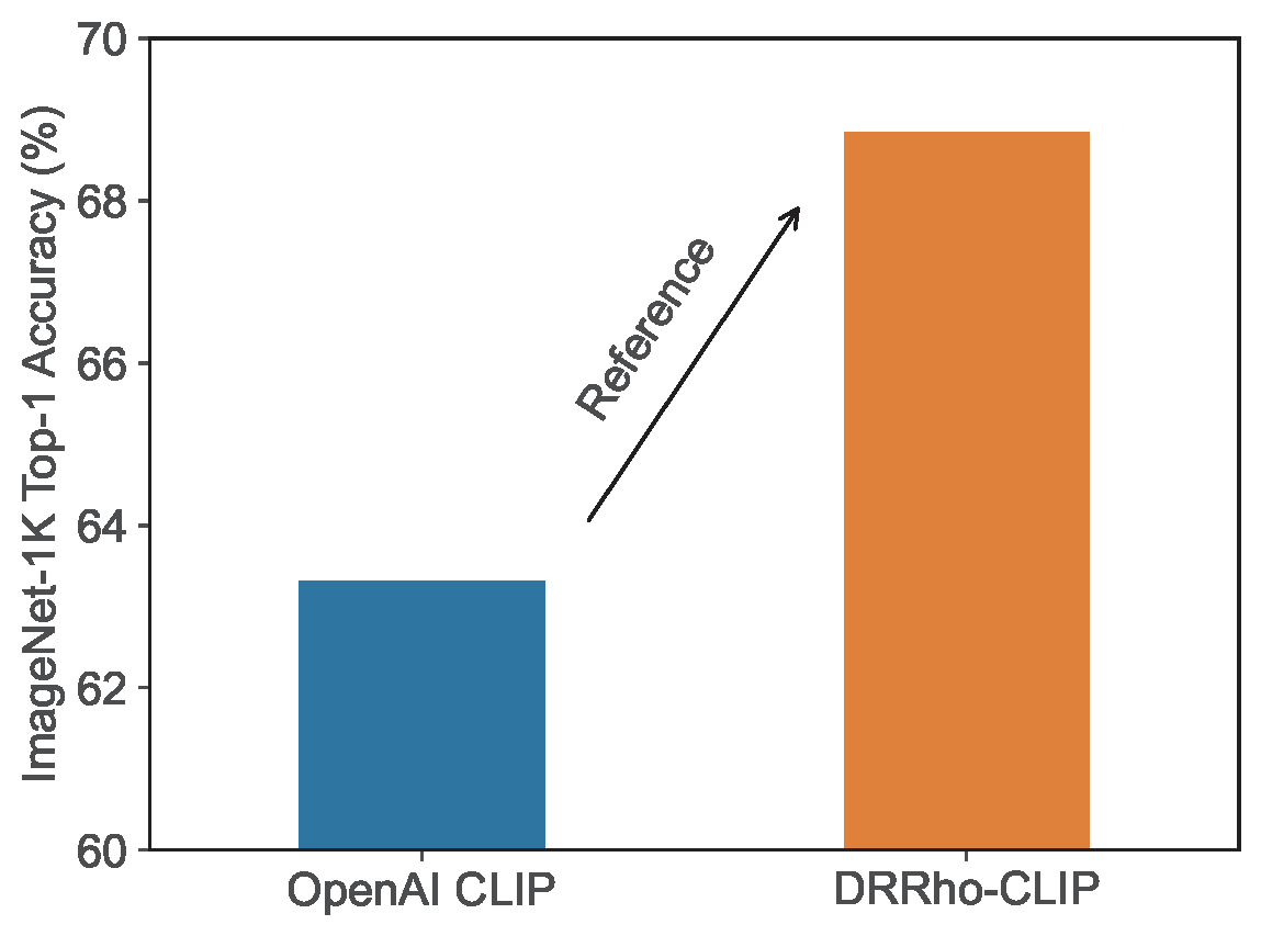
An emerging learning paradigm has recently surfaced that leverages a pre-trained reference model to guide and enhance training via strategic data weighting—a process we term reference model steering. Unlike the knowledge distillation framework, reference model steering does not assume that the reference model is a stronger teacher; in fact, it can lead to the training of a model that ultimately surpasses the reference model in performance, i.e., enabling weak to strong generalization.
DRRHO Risk Minimization
Let \(\mathbf{z} \sim \mathbb{P}\) denote a random data point drawn from distribution \(\mathbb{P}\), and let \(\mathbf{w} \in \mathcal{W}\) represent model parameters from a parameter space \(\mathcal{W}\). Given a loss function \(\ell(\mathbf{w}, \mathbf{z})\), the expected risk is defined as:
\[\mathcal{R}(\mathbf{w}) = \mathbb{E}_{\mathbf{z} \sim \mathbb{P}}[\ell(\mathbf{w}, \mathbf{z})].\]
Given a pretrained reference model \(\mathbf{w}_{\mathrm{ref}}\), we define a new loss \(\hat{\ell}(\mathbf{w}, \cdot) = \ell(\mathbf{w}, \cdot) - \ell(\mathbf{w}_{\mathrm{ref}}, \cdot)\), which is termed as RHO loss. Incorporating this into the distributionally robust optimization (DRO) framework, we define DRRHO risk minimization as:
\[\begin{equation}\label{eq:dro_ref_model} \min_{\mathbf{w} \in \mathcal{W}} \sup_{\mathbf{p} \in \Delta \atop D_{\phi}(\mathbf{p}\,\|\, 1/n) \le \rho / n} \sum_{i=1}^n p_i \left( \ell(\mathbf{w}, \mathbf{z}_i) - \ell(\mathbf{w}_{\mathrm{ref}}, \mathbf{z}_i) \right). \end{equation}\]
Theoretical guarantees for DRRHO have been developed with the \(\chi^2\) divergence, i.e., \(D_{\phi}(\mathbf{p}\,\|\, \mathbf{q}) = \sum_{i=1}^n \frac{1}{2} q_i \left( \frac{p_i}{q_i} - 1 \right)^2\). Under mild conditions, it can be shown that with high probability (Wei et al. 2025):
\[\begin{align}\label{eqn:drrho-e} \mathcal{R}(\tilde{\mathbf{w}}_*) \leq \inf_{\mathbf{w} \in \mathcal{W}} \left( \mathcal{R}(\mathbf{w}) + \sqrt{ \frac{2\rho}{n} \, \mathrm{Var}(\ell(\mathbf{w}, \cdot) - \ell(\mathbf{w}_{\mathrm{ref}}, \cdot)) } \right) + \mathcal{O}\left(\frac{1}{n}\right), \end{align}\]
where \(\tilde{\mathbf{w}}_*\) is an optimal solution to DRRHO risk minimization.
In particular, plugging in \(\mathbf{w}_* = \arg\min_{\mathbf{w} \in \mathcal{W}} \mathcal{R}(\mathbf{w})\) yields:
\[\mathcal{R}(\tilde{\mathbf{w}}_*) \leq \mathcal{R}(\mathbf{w}_*) + \sqrt{ \frac{2\rho}{n} \, \mathrm{Var}(\ell(\mathbf{w}_*, \cdot) - \ell(\mathbf{w}_{\mathrm{ref}}, \cdot)) } + \mathcal{O}\left(\frac{1}{n}\right).\]
This result provides valuable insight: if the reference model \(\mathbf{w}_{\mathrm{ref}}\) is well-trained such that \(\ell(\mathbf{w}_{\mathrm{ref}}, \cdot)\) closely matches \(\ell(\mathbf{w}_*, \cdot)\) in distribution, then the variance term becomes small. As a result, DRRHO achieves better generalization than the standard \(\mathcal{O}(\sqrt{1/n})\) bound of ERM.
Furthermore, if \(\mathbf{w}_{\mathrm{ref}} \in \mathcal{W}\), we obtain a comparison in terms of excess risk:
\[\mathcal{R}(\tilde{\mathbf{w}}_*) - \mathcal{R}(\mathbf{w}_*) \leq \mathcal{R}(\mathbf{w}_{\mathrm{ref}}) - \mathcal{R}(\mathbf{w}_*) + \mathcal{O}\left(\frac{1}{n}\right).\]
This enables a direct comparison between the DRRHO minimizer \(\tilde{\mathbf{w}}_*\) and the reference model \(\mathbf{w}_{\mathrm{ref}}\) from the same hypothesis class. Suppose \(\mathbf{w}_{\mathrm{ref}}\) was trained via ERM on a dataset with \(m\) samples. Then standard generalization theory gives an excess risk of order \(\mathcal{O}(1/\sqrt{m})\). In contrast, to match this level of generalization error, DRRHO requires only \(n = \mathcal{O}(\sqrt{m})\) samples—significantly improving over the \(\mathcal{O}(m)\) sample complexity required by ERM without a reference model.
Optimization Algorithms
When the CVaR is used defined by \(\phi(t) = 1\) if \(t \leq n/k\) and \(\phi(t) = \infty\) otherwise, the DRRHO risk reduces to the average of the top-\(k\) RHO losses:
\[\begin{align}\label{eqn:drrho1} \min_{\mathbf{w}} F(\mathbf{w}) := \frac{1}{k} \sum_{i=1}^k \left( \ell(\mathbf{w}, \mathbf{z}_{[i]}) - \ell(\mathbf{w}_{\mathrm{ref}}, \mathbf{z}_{[i]}) \right), \end{align}\]
where \(\mathbf{z}_{[i]}\) denotes the data point ranked \(i\)-th in descending order based on its RHO loss. This problem can be equivalently reformulated as:
\[\begin{align}\label{eqn:drrho1_equiv} \min_{\mathbf{w}, \nu} \;\frac{1}{k} \sum_{i=1}^n \left[ \ell(\mathbf{w}, \mathbf{z}_i) - \ell(\mathbf{w}_{\mathrm{ref}}, \mathbf{z}_i) - \nu \right]_+ + \nu, \end{align}\]
which is more amenable to gradient-based optimization techniques.
When DRRHO risk is defined using KL divergence regularization, the objective becomes:
\[\begin{align}\label{eqn:drrho3} \min_{\mathbf{w}} \;\tau \log\left( \frac{1}{n} \sum_{i=1}^n \exp\left( \frac{\ell(\mathbf{w}, \mathbf{z}_i) - \ell(\mathbf{w}_{\mathrm{ref}}, \mathbf{z}_i)}{\tau} \right) \right). \end{align}\]
This formulation can be optimized by simply replacing the loss in Algorithm 24 with the RHO loss. The vanilla gradient at iteration \(t\) is estimated by:
\[\frac{1}{B} \sum_{i \in \mathcal{B}_t} \frac{\exp\left( \frac{\ell(\mathbf{w}_t, \mathbf{z}_i) - \ell(\mathbf{w}_{\mathrm{ref}}, \mathbf{z}_i)}{\tau} \right)}{u_{t}} \nabla \ell(\mathbf{w}_t, \mathbf{z}_i),\]
where \(u_{t}\) is the MA estimator of the inner function value. This gradient estimator naturally assigns higher weights to data points with larger RHO losses, thereby prioritizing samples with high learnability during training.
Finally, when DRRHO is formulated with a KL-divergence constraint, the optimization problem becomes:
\[\begin{align}\label{eqn:drrho2} \min_{\mathbf{w}} \min_{\tau \geq 0} \; \tau \log\left( \frac{1}{n} \sum_{i=1}^n \exp\left( \frac{\ell(\mathbf{w}, \mathbf{z}_i) - \ell(\mathbf{w}_{\mathrm{ref}}, \mathbf{z}_i)}{\tau} \right) \right) + \frac{\tau \rho}{n}. \end{align}\]
This formulation can be optimized using techniques similar to those introduced in the first section of this chapter.
DRRHO-CLIP with a Reference Model
We now consider applying the DRRHO risk minimization framework to CLIP. Given the established connection between robust global contrastive loss and DRO, as shown here, it is straightforward to incorporate the RHO loss into the training objective. Define the following loss components:
\[\begin{align*} &\ell_1(\mathbf{w}; \mathbf{x}_i, \mathbf{t}_i, \mathbf{t}) = s(\mathbf{w}; \mathbf{x}_i, \mathbf{t}) - s(\mathbf{w}; \mathbf{x}_i, \mathbf{t}_i), \\ &\ell_2(\mathbf{w}; \mathbf{x}_i, \mathbf{t}_i, \mathbf{x}) = s(\mathbf{w}; \mathbf{x}, \mathbf{t}_i) - s(\mathbf{w}; \mathbf{x}_i, \mathbf{t}_i), \\ &\ell_1(\mathbf{w}_{\text{ref}}; \mathbf{x}_i, \mathbf{t}_i, \mathbf{t}) = s(\mathbf{w}_{\text{ref}}; \mathbf{x}_i, \mathbf{t}) - s(\mathbf{w}_{\text{ref}}; \mathbf{x}_i, \mathbf{t}_i), \\ &\ell_2(\mathbf{w}_{\text{ref}}; \mathbf{x}_i, \mathbf{t}_i, \mathbf{x}) = s(\mathbf{w}_{\text{ref}}; \mathbf{x}, \mathbf{t}_i) - s(\mathbf{w}_{\text{ref}}; \mathbf{x}_i, \mathbf{t}_i), \end{align*}\]
where \(s(\cdot; \cdot, \cdot)\) denotes the similarity function, and \(\mathbf{w}_{\text{ref}}\) is a pretrained reference model.
Using these definitions, we modify the original objective to incorporate the RHO loss:
\[\begin{equation}\label{eqn:drrho-clip} \begin{aligned} \min_{\mathbf{w}, \tau_1, \tau_2} \; &\frac{1}{n} \sum_{i=1}^n \tau_1 \log\left( \frac{1}{|\mathcal{T}^-_i|} \sum_{\mathbf{t} \in \mathcal{T}^-_i} \exp\left( \frac{\ell_1(\mathbf{w}; \mathbf{x}_i, \mathbf{t}_i, \mathbf{t}) - \ell_1(\mathbf{w}_{\text{ref}}; \mathbf{x}_i, \mathbf{t}_i, \mathbf{t})}{\tau_1} \right) \right) + \tau_1 \rho \\ +\; &\frac{1}{n} \sum_{i=1}^n \tau_2 \log\left( \frac{1}{|\mathcal{I}^-_i|} \sum_{\mathbf{x} \in \mathcal{I}^-_i} \exp\left( \frac{\ell_2(\mathbf{w}; \mathbf{x}_i, \mathbf{t}_i, \mathbf{x}) - \ell_2(\mathbf{w}_{\text{ref}}; \mathbf{x}_i, \mathbf{t}_i, \mathbf{x})}{\tau_2} \right) \right) + \tau_2 \rho. \end{aligned} \end{equation}\]
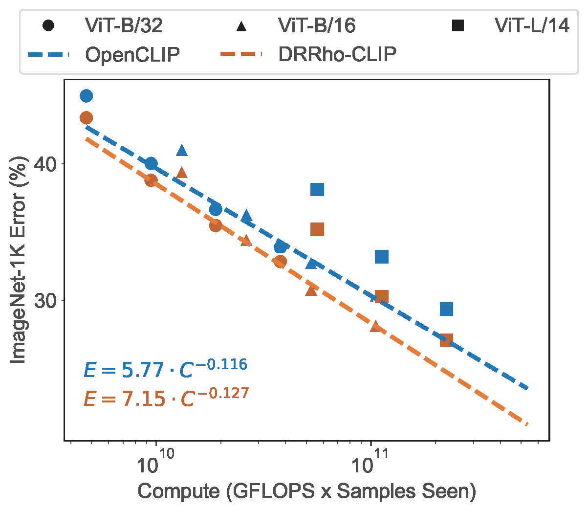
This objective can be optimized using an algorithm similar to that used in the CLIP training as presented in Section 6.5. Empirical results show that this approach significantly reduces sample complexity and improves the empirical scaling law (see Figure 6.33), while also achieving weak to strong generalization (see Figure 6.34).