Section 2.2 Robust Optimization
In this section, we introduce advanced machine learning methods based on the principle of robust optimization. Robust optimization is a framework designed to address uncertainty in data. It ensures that the solutions perform well even under worst-case scenarios of data within a specified set of uncertainties.
2.2.1 Distributionally Robust Optimization
Minimizing the average empirical risk often fails to yield a robust model in practice. For instance, the resulting model may perform poorly on minority data (e.g., patients with rare diseases) because the optimization predominantly focuses on majority class data.
To address these challenges, distributionally robust optimization (DRO) has been extensively studied in machine learning as a means to improve robustness and generalization.
The core idea of DRO is to minimize a robust objective defined over the worst-case distribution of data, perturbed from the empirical distribution. Let us define a set of distributional weights, \(\mathbf{p}=(p_1,\ldots,p_n)\in\Delta_n\), where \(\Delta_n=\{\mathbf{p}\in\mathbb{R}^n:\sum_{i=1}^n p_i=1,p_i\ge0\}\), with each element \(p_i\) associated with a training sample \(\mathbf{x}_i\).
Definition 2.1 (\(\phi\)-divergence).
Let \(\phi(t):\mathbb{R}^+\to\mathbb{R}\) be a
proper closed convex function and has a minimum value zero that is
attained at \(t=1\). The \(\phi\)-divergence is defined as: \[\begin{align}
D_{\phi}(\mathbf{p}\|\mathbf{q})=\sum_{i=1}^n q_i\phi(p_i/q_i).
\end{align}\]
\(\phi\)-divergence measures the discrepancy between two distributions \(\mathbf{p}\) and \(\mathbf{q}\) using the function \(\phi\). We present two common formulations of DRO based on the \(\phi\)-divergence: regularized DRO and constrained DRO. They differ in how to define the uncertainty set of \(\mathbf{p}\).
Below, we use the generic notation \(\ell(\mathbf{w};\mathbf{z})\) to denote the loss of a model \(\mathbf{w}\) on a random data point \(\mathbf{z}\) following a distribution denoted by \(\mathbb{P}\). For supervised learning, this specializes to \(\ell(\mathbf{w};\mathbf{z})=\ell(h(\mathbf{w};\mathbf{x}),y)\), where \(\mathbf{z}=(\mathbf{x},y)\).
Definition 2.2 (Regularized DRO).
\[\begin{align}\label{eqn:rdro}
\min_{\mathbf{w}}\hat{\mathcal{R}}_{\mathcal{S}}(\mathbf{w}):=\max_{\mathbf{p}\in\Delta_n}\sum_{i=1}^n
p_i\ell(\mathbf{w};\mathbf{z}_i)-\tau D_{\phi}\left(\mathbf{p}\|
\frac{\mathbf{1}}{n}\right).
\end{align}\]
Definition 2.3 (Constrained DRO).
\[\begin{align}\label{eqn:cdro}
\min_{\mathbf{w}}\hat{\mathcal{R}}_{\mathcal{S}}(\mathbf{w}):=&\max_{\mathbf{p}\in\Omega}\sum_{i=1}^n
p_i\ell(\mathbf{w};\mathbf{z}_i)\\
\text{where }&\quad\Omega=\left\{\mathbf{p}\mid
\mathbf{p}\in\Delta_n,D_{\phi}\left(\mathbf{p}\|
\frac{\mathbf{1}}{n}\right)\le\rho\right\}.\notag
\end{align}\]
The regularized DRO uses a regularization on the \(\mathbf{p}\) to implicitly define the uncertainty set, and the constrained DRO uses a constraint on \(\mathbf{p}\) to explicitly define the uncertainty set.
The maximization over \(\mathbf{p}\) in the DRO formulations simulates a worst-case scenario, thereby enhancing the model’s robustness. The DRO objective interpolates between the maximal loss and the average loss:
Without the \(\phi\)-divergence regularization or constraint (i.e., \(\tau=0\) or \(\rho=\infty\)), the objective simplifies to the maximal loss among all samples, which is particularly beneficial for handling imbalanced data but is sensitive to outliers.
Conversely, when \(\rho=0\) or \(\tau=\infty\), the DRO objective reduces to the standard empirical risk, which is not sensitive to outliers but not suitable for imbalanced data.
In practice, adding a tunable \(\phi\)-divergence regularization or constraint (via tuning \(\tau\) or \(\rho\)) increases the model’s robustness.
A list of \(\phi\)-divergence is presented in Table 2.1. Two commonly used ones in machine learning are presented below:
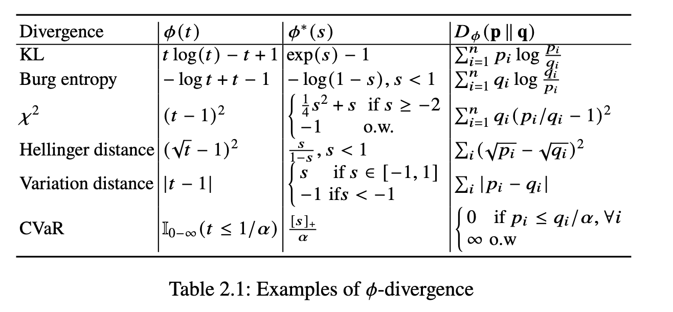
KL-Divergence: With \(\phi(t)=t\log t-t+1\), the \(\phi\)-divergence becomes the KL divergence: \[ \text{KL}(\mathbf{p},\mathbf{q})=D_{\phi}(\mathbf{p}\|\mathbf{q})=\sum_{i=1}^n p_i\log(p_i/q_i). \]
Conditional Value-at-Risk (CVaR): With \(\phi(t)=\mathbb{I}_{0-\infty}(t\le1/\alpha)\), where \(\alpha\in(0,1]\) and \(\mathbb{I}_{0-\infty}\) is \(0-\infty\) indicator function, the divergence becomes \(D_{\phi}(\mathbf{p}\|\mathbf{q})=0\) if \(p_i\le q_i/\alpha,\forall i\), otherwise \(D_{\phi}(\mathbf{p}\|\mathbf{q})=\infty\). The resulting DRO formulation is also known as the empirical CVaR-\(\alpha\).
The Dual form of Regularized DRO
Solving the above DRO formulations requires dealing with a high-dimensional variable \(\mathbf{p}\) from a simplex, which will incur additional overhead compared with solving ERM when the number of training data is large. The reason is that it requires performing a projection onto the simplex \(\Delta_n\) or the constrained simplex \(\Omega=\{\mathbf{p}\in\Delta_n,D_{\phi}\left(\mathbf{p}\| \frac{\mathbf{1}}{n}\right)\le\rho\}\). To reduce this overhead, one approach is to convert the problem into unconstrained one using the Langrangian dual theory based on the convex conjugate of \(\phi\) function.
Proposition 2.1 (Dual form of
Regularized DRO)
Let \(\phi^*(s)=\max_{t\ge0}ts-\phi(t)\). Then we
have
\[\begin{align}\label{eqn:dual-rdro} \max_{\mathbf{p}\in\Delta_n}\sum_{i=1}^n p_i\ell(\mathbf{w};\mathbf{z}_i)-\tau D_{\phi}\left(\mathbf{p}\| \frac{\mathbf{1}}{n}\right)=\min_{\nu}\frac{\tau}{n}\sum_{i=1}^n\phi^*\bigg(\frac{\ell(\mathbf{w};\mathbf{z}_i)-\nu}{\tau}\bigg)+\nu. \end{align}\]
The proof can be found in Example 1.14.
Example 2.1: KL-divergence Regularized DRO
For the special case of using KL-divergence, we can further simplify the above objective function. Since \(\phi(t)=t\log t-t+1\), then \(\phi^*(s)=\exp(s)-1\) (See Example 1.15) and solving \(\nu\) yields \[ \nu=\tau\log\bigg(\frac{1}{n}\sum_{i=1}^n\exp(\ell(\mathbf{w};\mathbf{z}_i)/\tau)\bigg). \] Plugging it back into the objective, we can obtain a simplified form \[ \max_{\mathbf{p}\in\Delta_n}\sum_{i=1}^n p_i\ell(\mathbf{w};\mathbf{z}_i)-\tau\text{KL}\left(\mathbf{p},\frac{\mathbf{1}}{n}\right) =\tau\log\bigg(\frac{1}{n}\sum_{i=1}^n\exp(\ell(\mathbf{w};\mathbf{z}_i)/\tau)\bigg). \] As a result, with \(\phi(t)=t\log t-t+1\), the KL-divergence regularized DRO (\(\ref{eqn:rdro}\)) is equivalent to
\[\begin{align}\label{eqn:klrdro} \min_{\mathbf{w}}\tau\log\left(\frac{1}{n}\sum_{i=1}^n\exp\left(\frac{\ell(\mathbf{w};\mathbf{z}_i)}{\tau}\right)\right). \end{align}\]
Example 2.2: Empirical CVaR
As another example, we derive the dual form of the empirical CVaR. With simple algebra, we can derive that \(\phi^*(s)=\frac{[s]_+}{\alpha}\) (See Example 1.15) for \(\phi(t)=\mathbb{I}_{0-\infty}(t\le1/\alpha)\).
As a result, with \(\phi(t)=\mathbb{I}_{0-\infty}(t\le1/\alpha)\), the regularized DRO (\(\ref{eqn:rdro}\)) corresponding to the empirical CVaR-\(\alpha\) is equivalent to
\[\begin{align}\label{eqn:cvar} \min_{\mathbf{w},\nu}\frac{1}{n\alpha}\sum_{i=1}^n[\ell(\mathbf{w};\mathbf{z}_i)-\nu]_+ + \nu. \end{align}\] When \(k=n\alpha\in[1,n]\) is an integer, the above objective reduces to the average of top-\(k\) loss values when sorting them in descending order, as shown in the following lemma.
Lemma 2.2
Let \(\ell_{[i]}\) denote the \(i\)-th largest loss among \(\{\ell(\mathbf{w};\mathbf{z}_i),i=1,\ldots,n\}\)
ranked in descending order. If \(\alpha=k/n\), we have \[\begin{align}\label{eqn:cvar-top-k}
\min_{\nu}\frac{1}{n\alpha}\sum_{i=1}^n[\ell(\mathbf{w};\mathbf{z}_i)-\nu]_+
+ \nu=\frac{1}{k}\sum_{i=1}^k\ell_{[i]}.
\end{align}\]
Proof.
First, we have \[
\min_{\nu}\frac{1}{n\alpha}\sum_{i=1}^n[\ell(\mathbf{w};\mathbf{z}_i)-\nu]_+
+ \nu
=\min_{\nu}\frac{1}{n\alpha}\sum_{i=1}^n[\ell_{[i]}-\nu]_+ + \nu.
\] Let \(\nu_*\) be an optimal
solution given \(\mathbf{w}\). Due to
the first-order optimality condition, we have \[\begin{align*}
0\in\frac{1}{k}\sum_{i=1}^n\partial_{\nu}[\ell_{[i]}-\nu_*]_+ + 1.
\end{align*}\] Hence, \[\begin{align}\label{eqn:opt-mu}
-k\in\sum_{i=1}^n\partial_{\nu}[\ell_{[i]}-\nu_*]_+.
\end{align}\] Let us first assume \(\ell_{[k+1]}<\ell_{[k]}\). We will show
that \(\nu_*\in(\ell_{[k+1]},\ell_{[k]}]\) satisfy
this condition. Since \(-1\in\partial_{\nu}[\ell_{[i]}-\nu_*]_+\)
for \(i=1,\ldots,k\) due to \(\ell_{[i]}\ge\nu_*\) and \(\partial_{\nu}[\ell_{[i]}-\nu_*]_+=0\) for
\(i=k+1,\ldots,n\) due to \(\ell_{[i]}<\nu_*\). Hence, it verifies
that the condition(\(\ref{eqn:opt-mu}\)) holds at such \(\nu_*\).
■
The Dual form of Constrained DRO
For transforming the constrained DRO, we can use the following proposition based on the Lagrangian duality theory.
Proposition 2.2 (Dual form of
Constrained DRO)
Let \(\phi^*(s)=\max_{t\ge0}ts-\phi(t)\). Then we
have
\[\begin{align}\label{eqn:dual-cdro} \max_{\mathbf{p}\in\Delta_n,D_{\phi}\left(\mathbf{p}\| \frac{\mathbf{1}}{n}\right)\le\rho}\sum_{i=1}^n p_i\ell(\mathbf{w};\mathbf{z}_i) =\min_{\tau\ge0,\nu}\frac{\tau}{n}\sum_{i=1}^n\phi^*\bigg(\frac{\ell(\mathbf{w};\mathbf{z}_i)-\nu}{\tau}\bigg)+\nu+\tau\rho. \end{align}\]
The proof is similar to that of Proposition 2.1.
Example 2.3: KL Constrained DRO
With \(\phi(t)=t\log t-t+1\), the KL-divergence constrained DRO (\(\ref{eqn:cdro}\)) is equivalent to:
\[\begin{align}\label{eqn:klcdro} \min_{\mathbf{w},\tau\ge0}\tau\log\left(\frac{1}{n}\sum_{i=1}^n\exp\left(\frac{\ell(\mathbf{w};\mathbf{z}_i)}{\tau}\right)\right)+\tau\rho. \end{align}\]
KL-regularized DRO and KL-constrained DRO play important roles in many modern artificial intelligence applications. The LDR loss can be interpreted as a form of KL-regularized DRO, except that the uncertainty is placed on the distribution of class labels for each individual data point. We will present additional applications in Section 2.4.
The Optimization Challenge
Although the transformed optimization problems do not involve dealing with a high-dimensional variable \(\mathbf{p}\in\Delta_n\), the new optimization problems (\(\ref{eqn:klrdro}\)), (\(\ref{eqn:klcdro}\)) are not of the same form as ERM. The critical assumption that an unbiased gradient can be easily computed fails. We will cast them as instances of stochastic compositional optimization (SCO), which is topic of Chapter 4 of the book.
2.2.2 Optimized Certainty Equivalent
How to understand the generalization of DRO? One way is to still consider bounding the expected risk \(\mathcal{R}(\mathbf{w})\) of the learned model. However, the expected risk may not be a good measure when the data distribution is skewed.
For simplicity, let us consider a binary classification problem with \(\Pr(\mathbf{x},y=1)=\pi_+\Pr(\mathbf{x}|y=1)\) and \(\Pr(\mathbf{x},y=-1)=\pi_-\Pr(\mathbf{x}|y=-1)\), where \(\pi_+=\Pr(y=1),\pi_-=\Pr(y=-1)\). Let \(\mathbb{P}_+\) and \(\mathbb{P}_-\) be the distributions of \(\mathbf{x}\) conditioned on \(y=1\) and \(y=-1\), respectively. By the law of total expectation we have \[\begin{align} \mathcal{R}(\mathbf{w})=\mathbb{E}_{\mathbf{x},y}\ell(h(\mathbf{w};\mathbf{x}),y) =\pi_+\mathbb{E}_{\mathbf{x}\sim\mathbb{P}_+}[\ell(h(\mathbf{w};\mathbf{x}),1)] +\pi_-\mathbb{E}_{\mathbf{x}\sim\mathbb{P}_-}[\ell(h(\mathbf{w};\mathbf{x}),-1)]. \end{align}\] If \(\pi_-\gg\pi_+\), the expected risk would be dominated by the expected loss of data from the negative class. As a result, a small \(\mathcal{R}(\mathbf{w})\) does not necessarily indicate a small \(\mathbb{E}_{\mathbf{x}\sim\mathbb{P}_+}[\ell(\mathbf{w};\mathbf{x},1)]\).
Instead, we consider the population risk of DRO as the target measure. A formal definition of the population risk for the regularized DRO(\(\ref{eqn:rdro}\)) is given below.
Definition 2.4 (Population risk of DRO).
Given a data distribution \(\mathbb{P}\), for any \(\tau>0\), we define the population risk
of regularized DRO (\(\ref{eqn:rdro}\))
as: \[\begin{align}
\mathcal{R}_{\text{oce}}(\mathbf{w}):=&\max_{\mathbb{Q}\in\mathcal{Q}}\mathbb{E}_{\mathbf{z}'\sim\mathbb{Q}}\ell(\mathbf{w};\mathbf{z}')-\tau\mathbb{E}_{\mathbb{P}}\phi\left(\frac{d\mathbb{Q}}{d\mathbb{P}}\right)\\
=&\min_{\nu}\tau\mathbb{E}_{\mathbf{z}\sim\mathbb{P}}\phi^*\left(\frac{\ell(\mathbf{w};\mathbf{z})-\nu}{\tau}\right)+\nu,\label{eqn:oce}
\end{align}\] where \(\phi^*(s)=\max_{t\ge0}ts-\phi(t)\).
In the definition above, \(\mathcal{Q}=\{\mathbb{Q}\mid \mathbb{Q}\ll \mathbb{P}\}\) denotes the set of probability measures that are absolutely continuous with respect to \(\mathbb{P}\). A probability measure \(\mathbb{Q}\) is said to be absolutely continuous with respect to \(\mathbb{P}\), denoted \(\mathbb{Q}\ll \mathbb{P}\), if every event that has probability \(0\) under \(\mathbb{P}\) also has probability \(0\) under \(\mathbb{Q}\). If \(\mathbb{P}\) and \(\mathbb{Q}\) admit densities \(p(z)\) and \(q(z)\) with respect to a common dominating measure on \(\mathcal{Z}\), and \(\mathbb{Q}\ll \mathbb{P}\), then \[ \mathbb{E}_{\mathbb{P}}\left[\phi\left(\frac{d\mathbb{Q}}{d\mathbb{P}}\right)\right] =\int_{\mathcal{Z}}p(z)\phi\left(\frac{q(z)}{p(z)}\right)\,dz. \]
The equivalent counterpart in (\(\ref{eqn:oce}\)) is a risk measure originates from the optimized certainty equivalent (OCE), a concept popularized in mathematical economics (Ben-Tal and Teboulle 2007). Minimizing OCE has an effect of so-called risk-aversion, which discourages models from having rare but catastrophic errors. Two special cases are discussed below:
When \(\phi(t)=\mathbb{I}_{0-\infty}(t\le1/\alpha)\), the OCE becomes the CVaR-\(\alpha\), i.e., \[ \mathcal{R}_{\text{cvar}}(\mathbf{w})=\mathbb{E}_{\mathbf{z}}[\ell(\mathbf{w};\mathbf{z})|\ell(\mathbf{w};\mathbf{z})\ge\text{VAR}_{\alpha}(\ell(\mathbf{w};\mathbf{z}))], \] where \(\text{VAR}_{\alpha}(\ell(\mathbf{w};\mathbf{z}))=\sup_s[\Pr(\ell(\mathbf{w};\mathbf{z})\ge s)\ge\alpha]\) is the \(\alpha\)-quantile or “value-at-risk” of the random loss values.
When \(\phi(t)=t\log t-t+1\), OCE becomes the entropic risk: \[ \mathcal{R}_{\text{ent}}(\mathbf{w})=\tau\log\left(\mathbb{E}_{\mathbf{z}}\exp\left(\frac{\ell(\mathbf{w};\mathbf{z})}{\tau}\right)\right). \]
We present two properties of OCE below.
Lemma 2.3
Let \(\partial\phi^*(t)=\{s:\phi'^{*}_-(t)\le
s\le\phi'^{*}_+(t)\}\). If \(a<b\), then \(0\le\phi'^*_+(a)\le\phi'^*_-(b)\).
Due to the definition \(\phi^*(s)=\max_{t\ge0}ts-\phi(t)\), we have \(\partial\phi^*(s)\ge0\), which indicates that \(\phi^*\) is non-decreasing. Since \(\phi^*\) is also convex, the conclusion follows from the convex analysis (Rockafellar, 1970).
■
Lemma 2.4
For any \(\tau>0,\mathbf{w}\in\mathbb{R}^d\), it
holds that \(\mathcal{R}_{\text{oce}}(\mathbf{w})\ge\mathcal{R}(\mathbf{w})\).
Since \(\phi(1)=0\), then \(\phi^*(s)=\max_{t\ge0}ts-\phi(t)\ge s-\phi(1)=s\). Hence, \[\begin{align*} \mathcal{R}_{\text{oce}}(\mathbf{w}) &=\min_{\nu}\tau\mathbb{E}_{\mathbf{z}}\phi^*\left(\frac{\ell(\mathbf{w};\mathbf{z})-\nu}{\tau}\right)+\nu\\ &\ge\min_{\nu}\tau\mathbb{E}_{\mathbf{z}}\left(\frac{\ell(\mathbf{w};\mathbf{z})-\nu}{\tau}\right)+\nu =\mathcal{R}(\mathbf{w}). \end{align*}\]
■
💡 Why it matters
Lemma 2.3 implies that a data with a larger
loss \(\ell(h(\mathbf{w};\mathbf{x}),y)\) will
have a higher weight in the gradient calculation in terms of \(\mathbf{w}\).
Lemma 2.4 indicates that OCE is a stronger measure than the expected risk. A small OCE will imply a small expected risk, while the reverse is not necessarily true.
Based on OCE, we can define the excess risk \(\mathcal{R}_{\text{oce}}(\mathbf{w})-\min_{\mathbf{u}\in\mathcal{W}}\mathcal{R}_{\text{oce}}(\mathbf{u})\) and decompose it into an optimization error and a generalization error similar to Lemma 2.1.
Lemma 2.5
For a learned model \(\mathbf{w}=\mathcal{A}(\mathcal{S};\zeta)\)
for solving empirical DRO (\(\ref{eqn:rdro}\)), we have \[\begin{align*}
\mathcal{R}_{\text{oce}}(\mathbf{w})-\min_{\mathbf{u}\in\mathcal{W}}\mathcal{R}_{\text{oce}}(\mathbf{u})
\le2\underbrace{\sup_{\mathbf{w}\in\mathcal{W}}|\mathcal{R}_{\text{oce}}(\mathbf{w})-\hat{\mathcal{R}}_{\mathcal{S}}(\mathbf{w})|}\limits_{\text{generalization
error}}
+\underbrace{\hat{\mathcal{R}}_{\mathcal{S}}(\mathbf{w})-\min_{\mathbf{u}\in\mathcal{W}}\hat{\mathcal{R}}_{\mathcal{S}}(\mathbf{u})}\limits_{\text{optimization
error}}.
\end{align*}\]
2.2.3 Group Distributionally Robust Optimization
Group DRO is an extension of DRO by aggregating data into groups and using DRO on the group level to formulate a robust risk function. It is helpful to promote equity of the learned model and mitigating the impact of spurious correlations that exist between the label and some features, by using prior knowledge to group the data.
Let us consider an illustrative example of classifying waterbird images from landbird images (see Figure 2.2). The training data may have the same number of waterbird images and landbird images. However, most waterbird images may have water in the background and most landbird images may have land in the background. Standard empirical risk minimization may learn spurious correlation between the class labels (e.g., waterbird) and the specific value of some attribute (e.g., the water background). As a consequence, the model may perform poorly on waterbird images with land background.
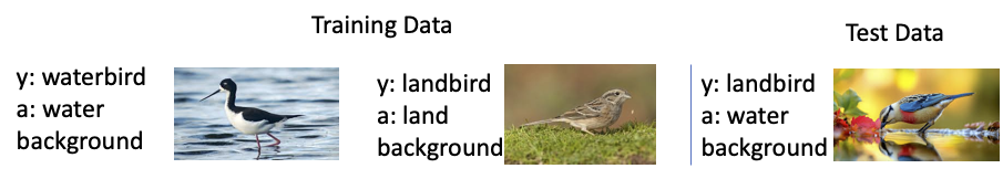
GDRO can be used to mitigate this issue by leveraging prior knowledge of spurious correlations to define groups over the training data. Let the training data be divided into multiple groups \(\mathcal{G}_1,\ldots,\mathcal{G}_K\), where \(\mathcal{G}_j=\{(\mathbf{x}^j_1,y^j_1),\ldots,(\mathbf{x}^j_{n_j},y^j_{n_j})\}\) includes a set of examples from the \(j\)-th group. We define an averaged loss over examples from each group \(L_j(\mathbf{w})=\frac{1}{n_j}\sum_{i=1}^{n_j}\ell(h(\mathbf{w};\mathbf{x}^j_i),y^j_i)\). Then, a regularized group DRO can be defined as \[\begin{align}\label{eqn:rgdro} \min_{\mathbf{w}}\max_{\mathbf{p}\in\Delta_K}\sum_{j=1}^K p_j L_j(\mathbf{w})-\tau D_{\phi}\left(\mathbf{p}\| \frac{\mathbf{1}}{K}\right), \end{align}\] and a constrained group DRO is given by: \[\begin{equation}\label{eqn:cgdro} \begin{aligned} \min_{\mathbf{w}}\max_{\mathbf{p}\in\Delta_K,D_{\phi}(\mathbf{p}\| \frac{\mathbf{1}}{K})\le\rho}\sum_{j=1}^K p_j L_j(\mathbf{w}). \end{aligned} \end{equation}\] By doing so, the learning process is less likely to be dominated by the majority group associated with the spurious correlation between the label and a particular feature (e.g., waterbird images with water background). If the model only captures the spurious correlation, the loss for the minority group will be large, which in turn drives the learning process to reduce this loss and thereby mitigate the spurious correlation.
Examples and Reformulations
Similar to before, we can convert the min-max problem into a minimization problem to reduce additional overhead of dealing with a large number of groups. We give two examples of using the KL-divergence constraint of \(\mathbf{p}\) and CVaR-\(\alpha\).
With \(\phi(t)=t\log t-t+1\), the KL-divergence constrained group DRO (\(\ref{eqn:cgdro}\)) is equivalent to \[\begin{align}\label{eqn:klgdro} \min_{\mathbf{w},\tau\ge0}\tau\log\left(\frac{1}{K}\sum_{j=1}^K\exp\left(\frac{L_j(\mathbf{w})}{\tau}\right)\right)+\tau\rho. \end{align}\] With \(\phi(t)=\mathbb{I}_{0-\infty}(t\le1/\alpha)\), CVaR-\(\alpha\) group DRO (\(\ref{eqn:cgdro}\)) is equivalent to \[\begin{align}\label{eqn:cvargdro} \min_{\mathbf{w},\nu}\frac{1}{K\alpha}\sum_{j=1}^K[L_j(\mathbf{w})-\nu]_+ + \nu. \end{align}\]
The Optimization Challenge
Again, these new optimization problems (\(\ref{eqn:klgdro}\)), (\(\ref{eqn:cvargdro}\)) cannot be solved by simply using existing stochastic algorithms for ERM since \(L_j(\mathbf{w})\) depends on many data and they are inside non-linear functions. In particular, the problem (\(\ref{eqn:cvargdro}\)) is an instance of finite-sum coupled compositional optimization (FCCO), which will be explored in Chapter 5 in depth.