Discriminative Data Prediction

The aforementioned X-risks can be unified under a principled discriminative learning framework for data prediction, providing a statistical foundation for developing advanced methods to train foundation models in modern AI.

The widely used foundation models include Contrastive Language-image Pretrained (CLIP) model (see Section 6.5), Dense Passage Retrieval (DPR) model, large language models (LLMs) such as the Generative Pretrained Transformer (GPT) series (see Section 6.6), and multi-modal large language models (MLLMs). These models fall into two main categories: representation models, such as CLIP and DPR, and generative models, including LLMs and MLLMs.

We present a discriminative data prediction framework to facilitate the learning of these foundation models. Suppose there exists a set of observed paired data, \(\{(\mathbf{x}_i,\mathbf{y}_i)\}_{i=1}^n\), where \(\mathbf{x}_i\in\mathcal{X}\) and \(\mathbf{y}_i\in\mathcal{Y}\). These pairs typically represent real-world positive correspondences. While this setup resembles traditional supervised learning where \(\mathbf{x}_i\) represents input data and \(\mathbf{y}_i\) denotes a class label, there is a crucial difference: here, \(\mathbf{y}_i\) refers to data from a continuous space (e.g., images with normalized pixel values) or a countably infinite space (e.g., text). For instance:

• In training the CLIP model, \(\mathbf{x}_i\) represents an image and \(\mathbf{y}_i\) is the corresponding text caption (or vice versa).

• In training the DPR model, \(\mathbf{x}_i\) is an input question, and \(\mathbf{y}_i\) is the corresponding textual answer.

• In fine-tuning LLMs or MLLMs, \(\mathbf{x}_i\) represents input data (e.g., prompts or images), and \(\mathbf{y}_i\) represents the text to be generated.

Since the risk function usually involves coupling each positive data with many other possibly negative data points in a compositional structure, the resulting risk is called discriminative X-risk. The following subsections detail two specific approaches to formulating discriminative X-risks.

A Discriminative Probabilistic Modeling Approach

Without loss of generality, we assume that \(\mathcal{X}\) and \(\mathcal{Y}\) are continuous spaces. Let \(\mathbb{P}_J\) denote the joint distribution of a pair \((\mathbf{x},\mathbf{y})\), and let \(\mathbb{P}_1\) and \(\mathbb{P}_2\) denote the marginal distributions of \(\mathbf{x}\) and \(\mathbf{y}\), respectively. We write their corresponding density functions as \(p(\cdot,\cdot)\), \(p_1(\cdot)\), and \(p_2(\cdot)\). We denote the conditional density functions by \(p(\mathbf{y}|\mathbf{x})\) and \(p(\mathbf{x}|\mathbf{y})\), corresponding to the conditional distributions \(\mathbb{P}(\mathbf{y}|\mathbf{x})\) and \(\mathbb{P}(\mathbf{x}|\mathbf{y})\). Below, we present two approaches based on discriminative probabilistic modeling (DPM).

Symmetric DPM

For symmetric DPM, we use \(s(\mathbf{w};\mathbf{x},\mathbf{y})\) to model both conditional distributions \(\mathbb{P}(\mathbf{y}|\mathbf{x})\) and \(\mathbb{P}(\mathbf{x}|\mathbf{y})\). A discriminative probabilistic approach models the conditional probability \(p(\mathbf{y}|\mathbf{x})\) using a scoring function \(s(\mathbf{w};\mathbf{x},\mathbf{y})\) by: \[\begin{align}\label{eqn:dpm} p_{\mathbf{w}}(\mathbf{y}|\mathbf{x})=\frac{p_2(\mathbf{y})\exp(s(\mathbf{w};\mathbf{x},\mathbf{y})/\tau)}{\int_{\mathbf{y}'\in\mathcal{Y}}p_2(\mathbf{y}')\exp(s(\mathbf{w};\mathbf{x},\mathbf{y}')/\tau)\,d\mathbf{y}'}, \end{align}\] where \(\tau>0\) is a temperature hyperparameter. The above parameterized distribution is the solution to the following problem for a fixed \(\mathbf{x}\): \[\begin{align*} p_{\mathbf{w}}(\cdot|\mathbf{x})=\arg\max_{\mathbb{Q}\in\mathcal{Q}}\mathbb{E}_{\mathbf{y}'\sim\mathbb{Q}}s(\mathbf{w};\mathbf{x},\mathbf{y}')-\tau\text{KL}(\mathbb{Q},\mathbb{P}_2), \end{align*}\] where \(\mathcal{Q}=\{\mathbb{Q}\mid\mathbb{Q}\ll\mathbb{P}_2\}\) is a set of probability distributions over \(\mathbf{y}\in\mathcal{Y}\).

Similarly, we model \(p(\mathbf{x}|\mathbf{y})\) as \[\begin{align}\label{eqn:dpm2} p_{\mathbf{w}}(\mathbf{x}|\mathbf{y})=\frac{p_1(\mathbf{x})\exp(s(\mathbf{w};\mathbf{x},\mathbf{y})/\tau)}{\int_{\mathbf{x}'\in\mathcal{X}}p_1(\mathbf{x}')\exp(s(\mathbf{w};\mathbf{x}',\mathbf{y})/\tau)\,d\mathbf{x}'}. \end{align}\]

Given a set of observed positive pairs \(\{(\mathbf{x}_i,\mathbf{y}_i)\}_{i=1}^n\), the model parameters \(\mathbf{w}\) are learned by minimizing the empirical risk of the negative log-likelihood: \[ \min_{\mathbf{w}}-\frac{1}{n}\sum_{i=1}^n\left\{\tau\log\frac{\exp(s(\mathbf{w};\mathbf{x}_i,\mathbf{y}_i)/\tau)}{\mathbb{E}_{\mathbf{y}'\sim\mathbb{P}_2}\exp(s(\mathbf{w};\mathbf{x}_i,\mathbf{y}')/\tau)}+\tau\log\frac{\exp(s(\mathbf{w};\mathbf{x}_i,\mathbf{y}_i)/\tau)}{\mathbb{E}_{\mathbf{x}'\sim\mathbb{P}_1}\exp(s(\mathbf{w};\mathbf{x}',\mathbf{y}_i)/\tau)}\right\}. \] A significant challenge in solving this problem lies in handling the partition functions, \[ Z(\mathbf{x}_i)=\mathbb{E}_{\mathbf{y}'\sim\mathbb{P}_2}\exp(s(\mathbf{w};\mathbf{x}_i,\mathbf{y}')/\tau),\quad Z(\mathbf{y}_i)=\mathbb{E}_{\mathbf{x}'\sim\mathbb{P}_1}\exp(s(\mathbf{w};\mathbf{x}',\mathbf{y}_i)/\tau), \] which are often computationally intractable. To overcome this, an approximation can be constructed using a set of samples \(\hat{\mathcal{Y}}_i\subseteq\mathcal{Y}\), \(\hat{\mathcal{X}}_i\subseteq\mathcal{X}\). The partition functions are then estimated by: \[ \hat{Z}(\mathbf{x}_i)=\frac{1}{|\hat{\mathcal{Y}}_i|}\sum_{\hat{\mathbf{y}}_j\in\hat{\mathcal{Y}}_i}\exp(s(\mathbf{w};\mathbf{x}_i,\hat{\mathbf{y}}_j)/\tau),\quad \hat{Z}(\mathbf{y}_i)=\frac{1}{|\hat{\mathcal{X}}_i|}\sum_{\hat{\mathbf{x}}_j\in\hat{\mathcal{X}}_i}\exp(s(\mathbf{w};\hat{\mathbf{x}}_j,\mathbf{y}_i)/\tau). \] Consequently, the resulting optimization problem is an empirical X-risk minimization problem: \[\begin{equation}\label{eqn:sym-dpm-exm} \begin{aligned} \min_{\mathbf{w}}\frac{1}{n}\sum_{i=1}^n\;&\tau\log\left(\sum_{\hat{\mathbf{y}}_j\in\hat{\mathcal{Y}}_i}\exp\left(\frac{s(\mathbf{w};\mathbf{x}_i,\hat{\mathbf{y}}_j)-s(\mathbf{w};\mathbf{x}_i,\mathbf{y}_i)}{\tau}\right)\right)\\ &+\tau\log\left(\sum_{\hat{\mathbf{x}}_j\in\hat{\mathcal{X}}_i}\exp\left(\frac{s(\mathbf{w};\hat{\mathbf{x}}_j,\mathbf{y}_i)-s(\mathbf{w};\mathbf{x}_i,\mathbf{y}_i)}{\tau}\right)\right). \end{aligned} \end{equation}\]

The above approach can be justified that if \(s(\mathbf{w},\cdot,\cdot)\) is optimized over all possible scoring functions, then the learned \(p_s(\mathbf{y}|\mathbf{x})\) and \(p_s(\mathbf{x}|\mathbf{y})\) approaches the true density functions of \(\mathbb{P}(\mathbf{y}|\mathbf{x})\) and \(\mathbb{P}(\mathbf{x}|\mathbf{y})\) when \(n\) approaches \(\infty\), respectively.

Proof.
Let \(\mathcal{F}_1\) be a class of functions \(f_1(\mathbf{x},\mathbf{y}):\mathcal{X}\times\mathcal{Y}\to\mathbb{R}\) such that \(f_1(\mathbf{x},\mathbf{y})\ge0\) and \(\int_{\mathbf{y}\in\mathcal{Y}}f_1(\mathbf{x},\mathbf{y})=1\), which induces a probability distribution \(\mathbb{Q}_{1,\mathbf{x}}(\cdot)\) over \(\mathcal{Y}\) for any \(\mathbf{x}\). Similarly, we define \(f_2(\mathbf{x},\mathbf{y})\in\mathcal{F}_2\) that induces a probability distribution \(\mathbb{Q}_{2,\mathbf{y}}(\cdot)\) over \(\mathcal{X}\) for any \(\mathbf{y}\).

■

One-sided DPM

If we are only interested in modeling \(\mathbb{P}(\mathbf{y}|\mathbf{x})\), then we can consider one-sided DPM. We define the following parametric probability function to model \(\mathbb{P}(\mathbf{y}|\mathbf{x})\): \[\begin{align} p_{\mathbf{w}}(\mathbf{y}|\mathbf{x})=\frac{\exp(s(\mathbf{w};\mathbf{x},\mathbf{y})/\tau)}{\int_{\mathcal{Y}}\exp(s(\mathbf{w};\mathbf{x},\mathbf{y}')/\tau)\,d\mu(\mathbf{y}')}, \end{align}\] where \(\tau>0\) is a temperature hyperparameter, and \(\mu\) is the Lebesgue measure associated with the space \(\mathcal{Y}\).

Given a set of observed positive pairs \(\{(\mathbf{x}_i,\mathbf{y}_i)\}_{i=1}^n\), the model parameters \(\mathbf{w}\) are learned by minimizing the empirical risk of the negative log-likelihood: \[ \min_{\mathbf{w}}-\frac{1}{n}\sum_{i=1}^n\tau\log\frac{\exp(s(\mathbf{w};\mathbf{x}_i,\mathbf{y}_i)/\tau)}{\int_{\mathcal{Y}}\exp(s(\mathbf{w};\mathbf{x}_i,\mathbf{y}')/\tau)\,d\mu(\mathbf{y}')}. \] A significant challenge in solving this problem lies in handling the partition function, \[ Z_i=\int_{\mathcal{Y}}\exp(s(\mathbf{w};\mathbf{x}_i,\mathbf{y}')/\tau)\,d\mu(\mathbf{y}'), \] which is often computationally intractable. To overcome this, an approximation can be constructed using a set of samples \(\hat{\mathcal{Y}}_i\subseteq\mathcal{Y}\). The partition function is then estimated as: \[ \hat{Z}_i=\sum_{\hat{\mathbf{y}}_j\in\hat{\mathcal{Y}}_i}\frac{1}{q_j}\exp(s(\mathbf{w};\mathbf{x}_i,\hat{\mathbf{y}}_j)/\tau), \] where \(q_j\) is an importance weight that accounts for the sample probability of \(\hat{\mathbf{y}}_j\). Consequently, the empirical X-risk minimization problem is reformulated as: \[ \min_{\mathbf{w}}\frac{1}{n}\sum_{i=1}^n\tau\log\left(\sum_{\hat{\mathbf{y}}_j\in\hat{\mathcal{Y}}_i}\exp\left(\frac{s(\mathbf{w};\mathbf{x}_i,\hat{\mathbf{y}}_j)+\zeta_j-s(\mathbf{w};\mathbf{x}_i,\mathbf{y}_i)}{\tau}\right)\right), \] where \(\zeta_j=\tau\ln\frac{1}{q_j}\).

We can similarly justify the above approach by the following theorem.

The proof is similar to the previous one and thus is omitted.

Instantiation

The fundamental difference between symmetric DPM and one-sided DPM lies in what their scoring functions \(s(\mathbf{w};\mathbf{x},\mathbf{y})\) are designed to capture. We can use symmetric DPM for learning representation models and one-sided DPM for learning generative models and supervised prediction models.

The standard cross-entropy loss for classification and the listwise cross-entropy loss for learning to rank can both be viewed as special cases of the one-sided DPM framework, where \(\mathcal{Y}\) represents either a finite set of class labels or a list of items to be ranked for each query. In these cases, the integral naturally simplifies to a finite summation, eliminating the need to approximate the normalization term \(Z_i\). However, when \(\mathcal{Y}\) is large, computing \(Z_i\) remains computationally demanding. This challenge, in turn, motivates the development of more advanced compositional optimization techniques.

For representation learning, the goal is to learn a symmetric scoring function \(s(\mathbf{w};\mathbf{x},\mathbf{y})=h_1(\mathbf{w};\mathbf{x})^{\top}h_2(\mathbf{w};\mathbf{y})\) that approximates the global optimum \[ s^{*}(\mathbf{x},\mathbf{y})=\tau\log\frac{p(\mathbf{x},\mathbf{y})}{p_1(\mathbf{x})p_2(\mathbf{y})}+\text{const}, \] which measures how much the joint distribution \(\mathbb{P}(\mathbf{x},\mathbf{y})\) deviates from independence between \(\mathbf{x}\) and \(\mathbf{y}\). We will consider contrastive losses of CLIP in Section 6.5 for multi-modal representation learning, which can be interpreted by the symmetric DPM with \(\mathbf{x},\mathbf{y}\) denoting an image-text pair.

For generative modeling, we can use underlying models to induce a scoring function \(s(\mathbf{w};\mathbf{x},\mathbf{y})\) for approximating the global optimum \(s^{*}(\mathbf{x},\mathbf{y})=\tau\log p(\mathbf{y}|\mathbf{x})+h(\mathbf{x})\). We will also consider discriminative fine-tuning of LLMs in Section 6.6, which can be interpreted by the one-sided DPM with \(\mathbf{x},\mathbf{y}\) denoting an input-output pair.

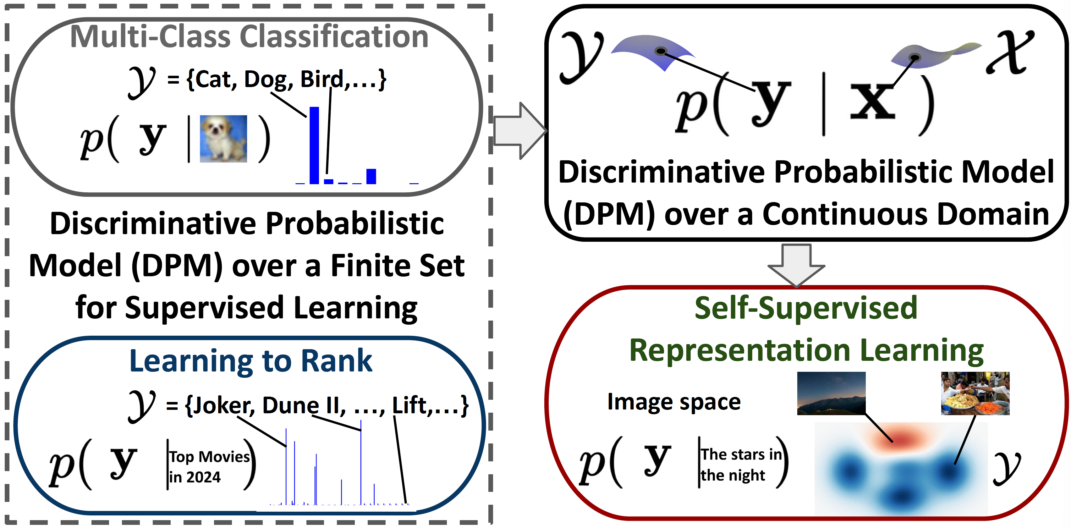
An illustration of the connection between the probabilistic model for multi-modal representation learning and traditional supervised learning tasks including multi-class classification and learning to rank is shown in Figure 2.5.

A Robust Optimization Approach

The goal of discriminative learning is to increase the score \(s(\mathbf{w};\mathbf{x},\mathbf{y}_+)\) for a “positive” pair \((\mathbf{x},\mathbf{y}_+)\) while decreasing the score \(s(\mathbf{w};\mathbf{x},\mathbf{y}_-)\) for any “negative” pair \((\mathbf{x},\mathbf{y}_-)\).

Full Supervised setting

Let us first consider the supervised learning setting, where positive and negative samples are labeled, i.e., there is a function \(r(\mathbf{x},\mathbf{y})\in(0,1)\) that indicates whether they form a positive pair or a negative pair. We let \((\mathbf{x},\mathbf{y}_+)\sim\mathbb{P}_+(\mathbf{x},\mathbf{y}_+)\) denote a positive pair and \((\mathbf{x},\mathbf{y}_-)\sim\mathbb{P}_-(\mathbf{x},\mathbf{y}_-)\) denote a negative pair, where \(\mathbb{P}_+(\mathbf{x},\mathbf{y}_+)=\mathbb{P}(\mathbf{x})\mathbb{P}_+(\mathbf{y}_+|\mathbf{x})\), \(\mathbb{P}_-(\mathbf{x},\mathbf{y}_-)=\mathbb{P}(\mathbf{x})\mathbb{P}_-(\mathbf{y}_-|\mathbf{x})\), and \(\mathbb{P}(\mathbf{x},\mathbf{y}_+,\mathbf{y}_-)=\mathbb{P}_+(\mathbf{y}_+|\mathbf{x})\mathbb{P}_-(\mathbf{y}_-|\mathbf{x})\mathbb{P}(\mathbf{x})\). Let us denote a pairwise loss by \(\ell(s(\mathbf{w};\mathbf{x},\mathbf{y}_-)-s(\mathbf{w};\mathbf{x},\mathbf{y}_+))\).

A naive goal is to minimize the expected risk: \[ \min_{\mathbf{w}}\mathbb{E}_{\mathbf{x},\mathbf{y}_+,\mathbf{y}_-\sim\mathbb{P}(\mathbf{x},\mathbf{y}_+,\mathbf{y}_-)}\big[\ell(s(\mathbf{w};\mathbf{x},\mathbf{y}_-)-s(\mathbf{w};\mathbf{x},\mathbf{y}_+))\big]. \] However, a fundamental challenge for data prediction is that the number of negative data is usually much larger than the number of positive data. Hence, the expected risk is not a strong measure. To address this challenge, we can leverage OCE. In particular, we replace the expected risk \(\mathbb{E}_{\mathbf{y}_-\sim\mathbb{P}(\mathbf{y}_-|\mathbf{x})}[\ell(s(\mathbf{w};\mathbf{x},\mathbf{y}_-)-s(\mathbf{w};\mathbf{x},\mathbf{y}_+))]\) by its OCE counterpart, resulting the following population risk: \[\begin{align}\label{eqn:soce-pop-1} \min_{\mathbf{w}}\mathbb{E}_{\mathbf{x},\mathbf{y}_+}\left[\min_{\nu}\tau\mathbb{E}_{\mathbf{y}_-|\mathbf{x}}\phi^*\left(\frac{\ell(s(\mathbf{w};\mathbf{x},\mathbf{y}_-)-s(\mathbf{w};\mathbf{x},\mathbf{y}_+))-\nu}{\tau}\right)+\nu\right]. \end{align}\] If the training dataset is \(\mathcal{S}=\{\mathbf{x}_i,\mathbf{y}_i^+,\mathbf{y}_{ij}^-,i\in[n],j\in[m]\}\), where \(\mathbf{y}_i^+\sim\mathbb{P}_+(\cdot|\mathbf{x}_i)\) and \(\mathbf{y}_{ij}^-\sim\mathbb{P}_-(\cdot|\mathbf{x}_i)\), then the empirical version becomes: \[\begin{align}\label{eqn:soce-1} \min_{\mathbf{w}}\frac{1}{n}\sum_{i=1}^n\min_{\nu_i}\tau\frac{1}{m}\sum_{j=1}^m\phi^*\left(\frac{\ell(s(\mathbf{w};\mathbf{x}_i,\mathbf{y}_{ij}^-)-s(\mathbf{w};\mathbf{x}_i,\mathbf{y}_i^+))-\nu_i}{\tau}\right)+\nu_i. \end{align}\]

Semi-supervised setting

We can extend the above framework to the semi-supervised learning setting, where we only have samples from the positive distribution \(\mathbb{P}_+(\cdot|\mathbf{x})\) and samples from the distribution \(\mathbb{P}(\cdot|\mathbf{x})\).

Let us assume that \(\mathbb{P}(\cdot|\mathbf{x})=\pi_+(\mathbf{x})\mathbb{P}_+(\cdot|\mathbf{x})+\pi_-(\mathbf{x})\mathbb{P}_-(\cdot|\mathbf{x})\) and \(\pi_+(\mathbf{x})\ll\pi_-(\mathbf{x})\). This means that for a fixed data \(\mathbf{x}\), the sampled data \(\mathbf{y}\sim\mathbb{P}(\cdot|\mathbf{x})\) is mostly likely from the negative distribution \(\mathbb{P}_-(\cdot|\mathbf{x})\). Hence, we can approximate \(\mathbb{E}_{\mathbf{y}_-\sim\mathbb{P}_-(\cdot|\mathbf{x})}\) by \(\mathbb{E}_{\mathbf{y}\sim\mathbb{P}(\cdot|\mathbf{x})}\). Hence, a population risk in the semi-supervised learning setting becomes \[\begin{align}\label{eqn:soce-pop-2} \min_{\mathbf{w}}\mathbb{E}_{\mathbf{x},\mathbf{y}_+}\left[\min_{\nu}\tau\mathbb{E}_{\mathbf{y}|\mathbf{x}}\phi^*\left(\frac{\ell(s(\mathbf{w};\mathbf{x},\mathbf{y})-s(\mathbf{w};\mathbf{x},\mathbf{y}_+))-\nu}{\tau}\right)+\nu\right], \end{align}\] and its empirical version becomes \[\begin{align}\label{eqn:soce-2} \min_{\mathbf{w}}\frac{1}{n}\sum_{i=1}^n\min_{\nu_i}\tau\frac{1}{m}\sum_{j=1}^m\phi^*\left(\frac{\ell(s(\mathbf{w};\mathbf{x}_i,\mathbf{y}_{ij})-s(\mathbf{w};\mathbf{x}_i,\mathbf{y}_i^+))-\nu_i}{\tau}\right)+\nu_i, \end{align}\] where \(\{\mathbf{y}_{ij},j=1,\ldots,m\}\) are samples from \(\mathbb{P}(\cdot|\mathbf{x})\).

Self-supervised setting

For self-supervised learning, we let \((\mathbf{x},\mathbf{y}^+)\sim\mathbb{P}(\mathbf{x},\mathbf{y}^+)\) denote a “positive” pair, and \((\mathbf{x},\mathbf{y}^-)\sim\mathbb{P}(\mathbf{x})\mathbb{P}(\mathbf{y}^-)\) denote a “negative” pair. For empirical learning, we only have a training set of \(\mathcal{S}=\{\mathbf{x}_i,\mathbf{y}_i^+,i\in[n]\}\). We use \(\mathcal{S}_i^-=\{\mathbf{y}_j^+\}_{j\ne i}\) to define the empirical risk: \[\begin{align}\label{eqn:soce-3} \min_{\mathbf{w}}\frac{1}{n}\sum_{i=1}^n\min_{\nu_i}\tau\frac{1}{|\mathcal{S}_i^-|}\sum_{\mathbf{y}'\in\mathcal{S}_i^-}\phi^*\left(\frac{\ell(s(\mathbf{w};\mathbf{x}_i,\mathbf{y}')-s(\mathbf{w};\mathbf{x}_i,\mathbf{y}_i^+))-\nu_i}{\tau}\right)+\nu_i. \end{align}\]

We refer to the problems in (\(\ref{eqn:soce-1}\)), (\(\ref{eqn:soce-2}\)) and (\(\ref{eqn:soce-3}\)) as the Compositional OCE (COCE) optimization. We will present and analyze stochastic algorithms for solving COCE optimization in Section 5.5.

Instantiation

When \(\phi(t)=t\log t-t+1\), the inner optimization over \(\nu_i\) in (\(\ref{eqn:soce-2}\)) admits a closed-form solution, which can be substituted back into the objective, yielding: \[\begin{align}\label{eqn:gcl-mu} \min_{\mathbf{w}}\frac{1}{n}\sum_{i=1}^n\tau\log\left(\frac{1}{m}\sum_{j=1}^m\exp\left(\frac{\ell(s(\mathbf{w};\mathbf{x}_i,\mathbf{y}_{ij})-s(\mathbf{w};\mathbf{x}_i,\mathbf{y}_i^+))}{\tau}\right)\right). \end{align}\] This formulation unifies several well-known losses as special cases:

• Cross-Entropy Loss for Classification: Let \(\mathbf{x}_i\) denote an input data point, let \(y_i^+\) represent its true class label and \(\{y_{ij},j=1,\ldots,m\}=\{1,\ldots,K\}\) forms the full label space. Define the prediction score for the \(y\)-th class of \(\mathbf{x}\) as \(s(\mathbf{w};\mathbf{x},y)=h_0(\mathbf{w}_0;\mathbf{x})^{\top}\mathbf{w}_y\). When the loss function is \(\ell(s)=s\) and \(\tau=1\), the objective reduces to the empirical risk with the standard cross-entropy loss.

• Listwise Cross-Entropy Loss for Ranking: Let \(\mathbf{x}_i\) denote a query, \(\{\mathbf{y}_i^+\}\) denote a relevant (positive) document, and \(\{\mathbf{y}_{ij}\}_{j=1}^m\) denote the complete candidate list to be ranked. Let \(s(\mathbf{w};\mathbf{x},\mathbf{y})\) be the predicted relevance score between a query \(\mathbf{x}\) and a document \(\mathbf{y}\). When the loss function is \(\ell(s)=s\) and \(\tau=1\), the objective simplifies to the listwise cross-entropy loss.

• Self-supervised Contrastive Loss for Representation Learning: If \(\mathbf{x}_i\) is an anchor (e.g., an image), \(\mathbf{y}_i^+\) denotes its positive pair (e.g., the corresponding text) and \(\{\mathbf{y}_{i,j},j=1,\ldots,m\}=\mathcal{S}_i^-\), the objective in (\(\ref{eqn:gcl-mu}\)) recovers the contrastive loss used in self-supervised contrastive representation learning.

• Partial AUC Loss for Imbalanced Binary Classification: Let \(\mathbf{x}_i\) be a fixed class label (\(i=1\)), with \(\{\mathbf{y}_i^+\}\) denoting its positive data set and \(\{\mathbf{y}_{ij}\}_{j=1}^m\) being its negative data set. Define the scoring function as \(s(\mathbf{w};\mathbf{x},\mathbf{y})=h(\mathbf{w};\mathbf{y})\in\mathbb{R}\). Under this setting, the objective in (\(\ref{eqn:gcl-mu}\)) reduces to the partial AUC loss.

This framework offers a flexible foundation for designing alternative robust objectives by varying the loss function \(\ell(\cdot)\), the temperature \(\tau\), the divergence function \(\phi(\cdot)\), and the distributionally robust optimization (DRO) formulation, including its constrained variants.

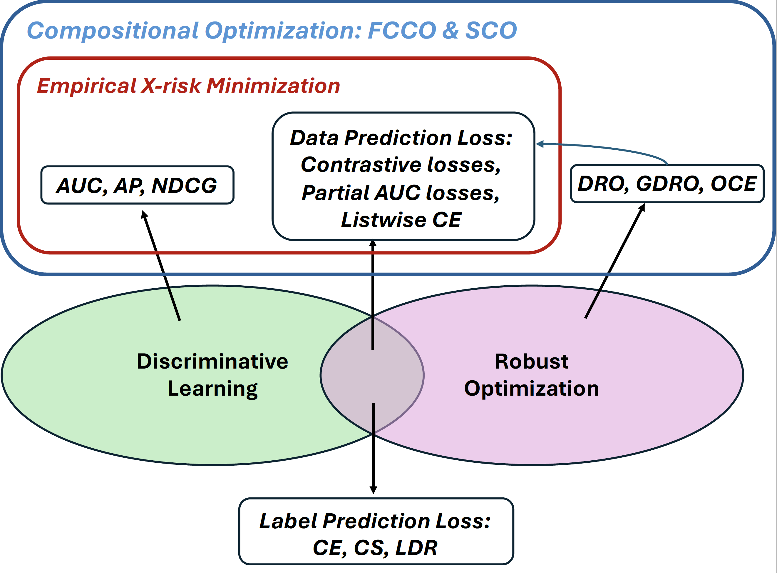
Finally, Figure 2.6 illustrates the losses, objectives, and learning frameworks discussed in this chapter, along with their connections to the principles of discriminative learning and robust optimization. This perspective highlights the necessity of stochastic compositional optimization and finite-sum coupled compositional optimization, which will be presented in subsequent chapters.

← Go Back