Section 2.3 Empirical X-risk Minimization

So far, we have revisited classical ideas of machine learning based on empirical risk minimization and its distributionally robust variant. In these risk functions, we assume each data point defines a loss based on itself. These losses are typically surrogate functions of a prediction error measuring the inconsistency between the prediction and the label.

However, such loss functions are insufficient to capture many objectives that involve comparisons between different data points. Examples include areas under ROC curves (AUROC) and areas under precision-recall curves (AUPRC) for imbalanced data classification, ranking measures such as normalized discounted cumulative gain (NDCG), mean average precision (MAP), and listwise losses for learning to rank, as well as contrastive losses for representation learning.

The standard ERM framework is inadequate for optimizing such metrics and losses, as they involve interactions across multiple data points. We need a new mathematical framework to understand the challenge and to design provable and practical algorithms. To this end, we introduce a new risk minimization framework, named empirical X-risk minimization (EXM), as defined below.

With \(g\) given in (\(\ref{eqn:avg-g}\)), EXM is an instance of finite-sum coupled compositional optimization (FCCO), which is the focus of Chapter 5.

2.3.1 AUC Losses

Areas under ROC curves (AUC) are commonly used to measure performance for imbalanced data classification.

What is Imbalanced Data Classification?

Imbalanced data classification refers to classification problems where the number of examples from some classes is significantly larger than that of other classes.

---

Definition and an Empirical Estimator of AUC

The ROC curve is the plot of the true positive rate (TPR) against the false positive rate (FPR) at each threshold setting. Let \(P_+, P_-\) denote the distributions of random positive and negative data, respectively. Let \(h(\cdot)\) denote a predictive function. For a given threshold \(t\), the TPR of \(h\) can be written as \(\text{TPR}(t) = \Pr(h(\mathbf x) > t | y = 1) = \mathbb E_{\mathbf x \sim P_+}[\mathbb I(h(\mathbf x) > t)]\), and the FPR can be written as
\(\text{FPR}(t) = \Pr(h(\mathbf x) > t | y = -1) = \mathbb E_{\mathbf x \sim P_-}[\mathbb I(h(\mathbf x) > t)]\).

Let \(F_-(t) = 1 - \text{FPR}(t)\) denote the cumulative density function of the random variable \(h(\mathbf x_-)\) for \(\mathbf x_- \sim P_-\). Let \(p_-(t)\) denote its corresponding probability density function. Similarly, let \(F_+(t) = 1 - \text{TPR}(t)\) and \(p_+(t)\) denote the cumulative density function and probability density function of \(h(\mathbf x_+)\) for \(\mathbf x_+ \sim P_+\), respectively. For a given \(u \in [0, 1]\), let \(\text{FPR}^{-1}(u) = \inf\{t \in R : \text{FPR}(t) \le u\}\). The ROC curve is defined as \(\{u, \text{ROC}(u)\}\), where \(u \in [0, 1]\) and \(\text{ROC}(u) = \text{TPR}(\text{FPR}^{-1}(u))\).

Proof.

The AUC score of \(h\) is given by

\[\begin{align*} \text{AUC}(h) &= \int_0^1 \text{ROC}(u) \, du = \int_{-\infty}^{\infty} \text{TPR}(t) \, dF_-(t) = \int_{-\infty}^{\infty} \text{TPR}(t) p_-(t) \, dt \notag \\ &= \int_{-\infty}^{\infty} \int_t^{\infty} p_+(s) \, ds \, p_-(t) \, dt = \int_{-\infty}^{\infty} \int_{-\infty}^{\infty} p_+(s) p_-(t) \mathbb I(s > t) \, ds \, dt. \end{align*}\]

Since \(h(\mathbf x_+)\) follows \(p_+(s)\) and \(h(\mathbf x_-)\) follows \(p_-(t)\), we can conclude the proof. ∎

This indicates that AUC is a pairwise ranking metric. An ideal predictive function that ranks all positive examples above negative examples has a perfect AUC score of \(1\).

It also implies the following empirical non-parametric estimator of AUC based on a set of data \(S\) with \(n_+\) positive samples in \(S_+\) and \(n_-\) negative samples in \(S_-\):

\[\begin{align}\label{eqn:auc-emp} \text{AUC}(h; S) = \frac{1}{n_+ n_-} \sum_{\mathbf x_+ \in S_+, \, \mathbf x_- \in S_-} \mathbb I(h(\mathbf x_+) > h(\mathbf x_-)), \end{align}\]

which is also known as the Mann–Whitney U-statistic.

Necessity of Maximizing AUC

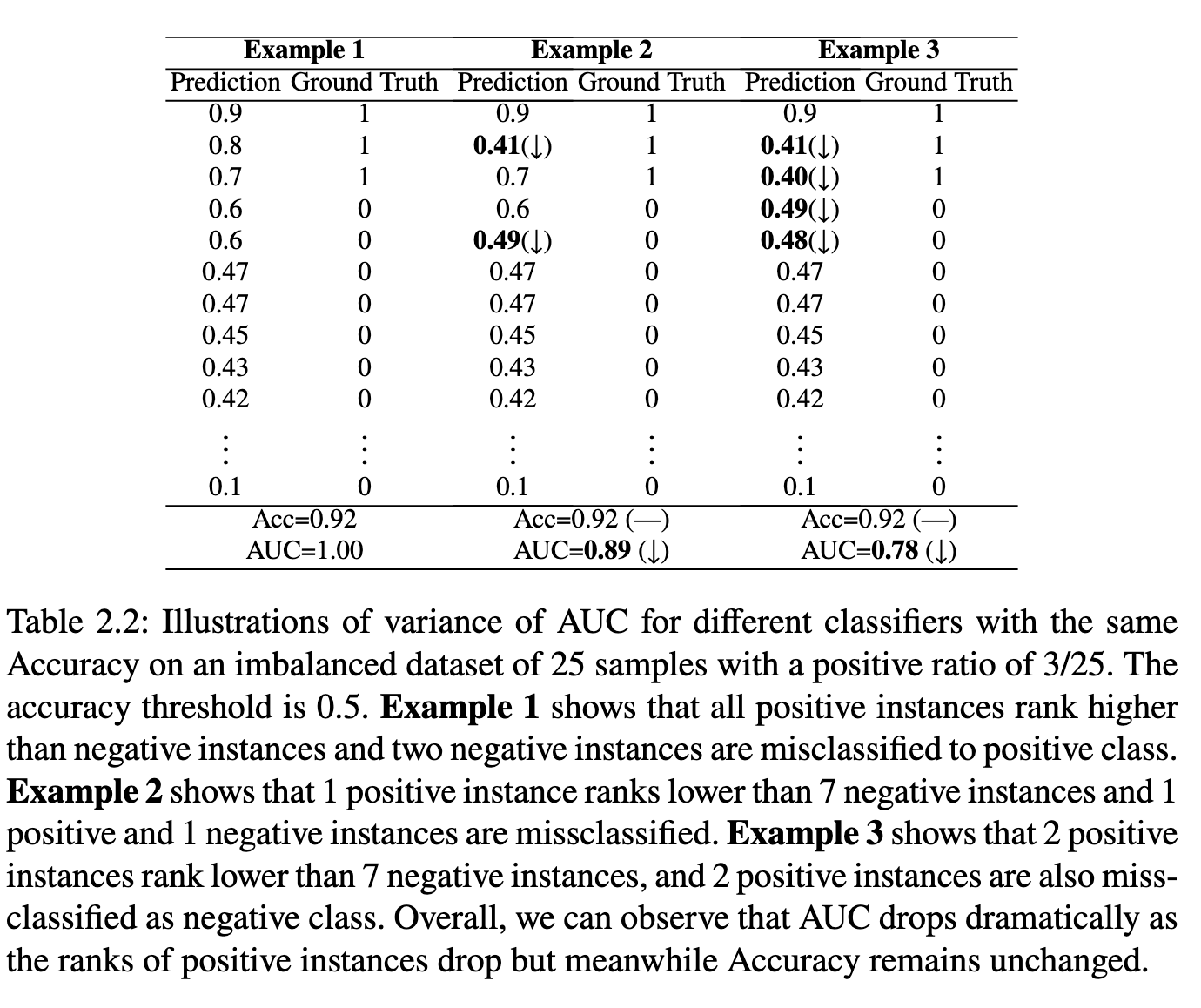
AUC is more appropriate than accuracy for assessing performance in imbalanced data classification. Consider an example with two positive data points and 100 negative data points. If one positive sample has a prediction score of \(0.5\) and the other \(-0.2\), and all negative samples have prediction scores less than \(0\) but greater than \(-0.2\), then with a classification threshold of \(0\), the accuracy is \(101/102 = 0.99\). However, the empirical AUC score according to (\(\ref{eqn:auc-emp}\)) is given by \(100/200 = 0.5\).

Can a model that optimizes accuracy also optimize the AUC score? Unfortunately, this is not the case, as different classifiers with the same accuracy may have dramatically different AUC values. An illustrative example is shown in the Table 2.2. Hence, it makes sense to directly optimize AUC.

Critical: A model that optimizes accuracy does not necessarily optimize AUC.

Pairwise Surrogate Losses

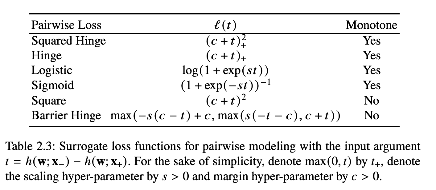
Using a pairwise surrogate loss \(\ell(\cdot)\) of the indicator function (see examples in Table 2.3), we have the following empirical AUC optimization problem for learning a parameterized function \(h(\mathbf{w}; \cdot)\):

\[\begin{align}\label{eqn:eaucd} \min_{\mathbf{w} \in \mathbb{R}^d} \frac{1}{n_+}\frac{1}{n_-}\sum_{\mathbf{x}_i \in \mathcal{S}_+}\sum_{\mathbf{x}_j \in \mathcal{S}_-}\ell\big(h(\mathbf{w}; \mathbf{x}_j) - h(\mathbf{w}; \mathbf{x}_i)\big). \end{align}\]

This can be regarded as a special case of (\(\ref{eqn:xrisk}\)) by setting

\[ \begin{aligned} &g(\mathbf{w}; \mathbf{x}_i, \mathcal{S}_-) = \frac{1}{n_-}\sum_{\mathbf{x}_j \in \mathcal{S}_-}\ell\big(h(\mathbf{w}; \mathbf{x}_j) - h(\mathbf{w}; \mathbf{x}_i)\big),\\ &f_i(g) = g. \end{aligned} \]

This is the simplest form of EXM since \(f\) is just a linear function. An unbiased stochastic gradient can be easily computed based on a pair of data points consisting of a random positive and a random negative data point.

Compositional Objectives

An alternative approach to formulate AUC maximization is to decouple the pairwise comparison between positive and negative examples. A generic formulation is given by:

\[\begin{equation}\label{eqn:aucminmax} \begin{aligned} \min_{\mathbf{w} \in \mathbb{R}^d, (a,b) \in \mathbb{R}^2}\quad & \frac{1}{|\mathcal{S}_+|}\sum_{\mathbf{x}_i \in \mathcal{S}_+}\big(h(\mathbf{w}; \mathbf{x}_i) - a\big)^2 + \frac{1}{|\mathcal{S}_-|}\sum_{\mathbf{x}_j \in \mathcal{S}_-}\big(h(\mathbf{w}; \mathbf{x}_j) - b\big)^2 \\ &\quad + f\!\left(\frac{1}{|\mathcal{S}_-|}\sum_{\mathbf{x}_j \in \mathcal{S}_-} h(\mathbf{w}; \mathbf{x}_j) - \frac{1}{|\mathcal{S}_+|}\sum_{\mathbf{x}_i \in \mathcal{S}_+} h(\mathbf{w}; \mathbf{x}_i)\right), \end{aligned} \end{equation}\]

where \(f\) is a non-linear function. The last component is a compositional function.

The above formulation also has a clear physical meaning. The first two terms push the prediction scores of positive and negative examples to center around their respective means, and the third term pushes the mean score of positive examples to be larger than that of negative examples.

This formulation is motivated by the pairwise formulation with a square surrogate function \(\ell\big(h(\mathbf{w}; \mathbf{x}_j) - h(\mathbf{w}; \mathbf{x}_i)\big) = \big(c + h(\mathbf{w}; \mathbf{x}_j) - h(\mathbf{w}; \mathbf{x}_i)\big)^2\). Indeed, in this case, (\(\ref{eqn:eaucd}\)) is equivalent to (\(\ref{eqn:aucminmax}\)) with \(f(s) = (s + c)^2\). Nevertheless, using \(f(s) = [s + c]_+^2\) in (\(\ref{eqn:aucminmax}\)) is more robust than \(f(s) = (s + c)^2\) with \(c > 0\).

Solving the above problem requires compositional optimization techniques, which will be discussed in Section 6.3.

2.3.2 Average Precision Loss

Area under the precision-recall curve (AUPRC) is another commonly used measure for highly imbalanced data. AUPRC is an average of the precision weighted by the probability of a given threshold, which can be expressed as:

\[ \text{AUPRC} = \int_{-\infty}^{\infty} \Pr(y = 1 \mid h(\mathbf{x}) \ge t) \, d\Pr(h(\mathbf{x}) \le t \mid y = 1), \]

where \(\Pr(y = 1 \mid h(\mathbf{x}) \ge t)\) is the precision at threshold \(t\).
For a set of training examples \(\mathcal{S} = \mathcal{S}_+ \cup \mathcal{S}_-\), a non-parametric estimator of AUPRC is the average precision (AP):

\[\begin{align}\label{eqn:AP} \text{AP} = \frac{1}{n_+} \sum_{\mathbf{x}_i \in \mathcal{S}_+} \frac{\sum_{\mathbf{x}_j \in \mathcal{S}_+} \mathbb{I}(h(\mathbf{x}_j) \ge h(\mathbf{x}_i))}{ \sum_{\mathbf{x}_j \in \mathcal{S}} \mathbb{I}(h(\mathbf{x}_j) \ge h(\mathbf{x}_i))}. \end{align}\]

AP is an unbiased estimator of AUPRC in the limit \(n \to \infty\).

Necessity of Maximizing AUPRC

While AUC is generally more suitable than accuracy for imbalanced classification tasks, it may fail to adequately capture misorderings among top-ranked examples.

Let us consider a scenario with two positive and 100 negative samples. If the two positive samples are ranked below only two of the negative ones, followed by the remaining 98 negatives, the resulting AUC is \(196/200 = 0.98\), which appears high. However, this model would be inadequate if our focus is on the top two predicted positive instances.

In domains such as drug discovery, models are expected to identify the most promising candidate molecules for experimental validation. If these top-ranked predictions turn out to lack the desired properties, the resulting experimental efforts may lead to significant wasted resources and costly failures.

To avoid this issue, AUPRC or its empirical estimator, average precision (AP), is typically used as a performance metric. According to its definition (\(\ref{eqn:AP}\)), the AP score for the above example is \(\frac{1}{2} \left(\frac{1}{3} + \frac{2}{4}\right) = 0.42\).
In contrast, a perfect ranking that places the two positive examples at the top gives an AP score of \(1\).

Unfortunately, optimizing AUC does not necessarily lead to optimal AP, as two models with identical AUC scores can exhibit significantly different AP values. This highlights the need for efficient optimization algorithms that directly maximize AP.

Critical: AUPRC/AP penalizes errors at the top of the ranked list more heavily.

Surrogate Loss of AP

To construct a differentiable objective for minimization, a differentiable surrogate loss \(\ell(h(\mathbf{x}_j) - h(\mathbf{x}_i))\) (cf. Table 2.3) is used in place of \(\mathbb{I}(h(\mathbf{x}_j) \ge h(\mathbf{x}_i))\).
Then, AP can be approximated by:

\[\begin{align}\label{eqn:AP-app} \text{AP} \approx \frac{1}{n_+} \sum_{\mathbf{x}_i \in \mathcal{S}_+} \frac{\sum_{\mathbf{x}_j \in \mathcal{S}} \mathbb{I}(y_j = 1)\ell(h(\mathbf{x}_j) - h(\mathbf{x}_i))}{ \sum_{\mathbf{x}_j \in \mathcal{S}} \ell(h(\mathbf{x}_j) - h(\mathbf{x}_i))}. \end{align}\]

Let us define:

\[ \begin{aligned} &f(\mathbf{g}) = -\frac{[\mathbf{g}]_1}{[\mathbf{g}]_2}, \\ &\mathbf{g}(\mathbf{w}; \mathbf{x}_i, \mathcal{S}) = [g_1(\mathbf{w}; \mathbf{x}_i, \mathcal{S}), g_2(\mathbf{w}; \mathbf{x}_i, \mathcal{S})], \\ &g_1(\mathbf{w}; \mathbf{x}_i, \mathcal{S}) = \frac{1}{|\mathcal{S}|}\sum_{\mathbf{x}_j \in \mathcal{S}} \mathbb{I}(y_j = 1)\ell(h(\mathbf{w}; \mathbf{x}_j) - h(\mathbf{w}; \mathbf{x}_i)), \\ &g_2(\mathbf{w}; \mathbf{x}_i, \mathcal{S}) = \frac{1}{|\mathcal{S}|}\sum_{\mathbf{x}_j \in \mathcal{S}} \ell(h(\mathbf{w}; \mathbf{x}_j) - h(\mathbf{w}; \mathbf{x}_i)). \end{aligned} \]

Then, we can formulate AP maximization as the following problem:

\[\begin{align}\label{eqn:apsurr} \min_{\mathbf{w}} \frac{1}{n_+} \sum_{\mathbf{x}_i \in \mathcal{S}_+} f(\mathbf{g}(\mathbf{w}; \mathbf{x}_i, \mathcal{S})), \end{align}\]

which is a special case of EXM. We will explore efficient algorithms for optimizing AP in Section 6.3 using FCCO techniques.

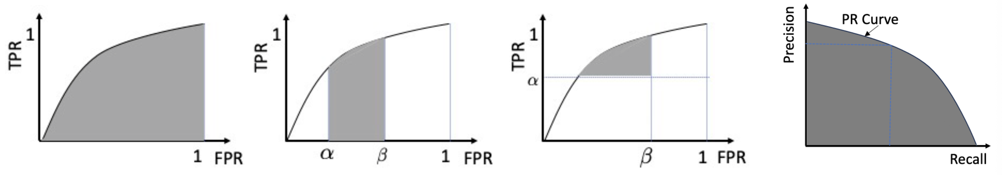
2.3.3 Partial AUC Losses

There are two commonly used versions of partial AUC (pAUC), namely one-way pAUC (OPAUC) and two-way pAUC (TPAUC). OPAUC puts a restriction on the range of FPR, i.e., \(\text{FPR} \in [\alpha, \beta]\) (see Figure 2.3, middle), and TPAUC puts a restriction on the lower bound of TPR and the upper bound of FPR, i.e., \(\text{TPR} \ge \alpha\), \(\text{FPR} \le \beta\) (see Figure 2.3, right).

Proof. The first part (OPAUC) parallels the AUC derivation but restricts the range of integration: \[\begin{align*} \text{OPAUC}(h \mid \text{FPR} \in (\alpha, \beta)) &= \int_{\text{FPR}^{-1}(\beta)}^{\text{FPR}^{-1}(\alpha)} \text{TPR}(t)\, dF_-(t) \\ &= \int_{\text{FPR}^{-1}(\beta)}^{\text{FPR}^{-1}(\alpha)} \int_{-\infty}^{\infty} p_+ (s)\, p_-(t)\, \mathbb{I}(s > t)\, ds\, dt. \end{align*}\] This proves the first claim.

For TPAUC with FPR restricted to \([0, \beta]\) and TPR restricted to \([\alpha, 1]\), it can be expressed as the difference between two OPAUC regions — one with \(\text{FPR} \in [\gamma, \beta]\) and another representing the square area with \(\text{TPR} < \alpha\), where \(\gamma\) corresponds to \(\text{TPR} = \alpha\), i.e., \(\text{FPR}^{-1}(\gamma) = \text{TPR}^{-1}(\alpha)\). Given that \(\text{TPR}(t) = \int_t^{\infty} p_+(s) ds\) and \(\text{FPR}(t) = \int_t^{\infty} p_-(s) ds\), we have:

\[ \alpha = \int_{\text{TPR}^{-1}(\alpha)}^{\infty} p_+(s) ds, \quad \beta = \int_{\text{FPR}^{-1}(\beta)}^{\infty} p_-(t) dt. \]

Then,

\[ \begin{aligned} (\beta - \gamma)\alpha &= \int_{\text{FPR}^{-1}(\beta)}^{\text{FPR}^{-1}(\gamma)} \int_{\text{TPR}^{-1}(\alpha)}^{\infty} p_+(s) p_-(t) \, ds \, dt, \end{aligned} \]

and thus,

\[ \begin{aligned} \text{TPAUC}(h \mid \text{TPR} \ge \alpha, \text{FPR} \le \beta) &= \text{OPAUC}(h, \gamma, \beta) - (\beta - \gamma)\alpha \\ &= \int_{\text{FPR}^{-1}(\beta)}^{\text{FPR}^{-1}(\gamma)} \int_t^{\text{TPR}^{-1}(\alpha)} p_+(s) p_-(t) \, ds \, dt \\ &= \int_{\text{FPR}^{-1}(\beta)}^{\infty} \int_t^{\text{TPR}^{-1}(\alpha)} p_+(s) p_-(t) \, ds \, dt. \end{aligned} \]

This completes the proof. ∎

Hence, an empirical estimator of OPAUC with \(\text{FPR} \in [\alpha,\beta]\) can be computed by

\[\begin{align}\label{eqn:opauc-emp} \frac{1}{n_+ k_1}\sum_{\mathbf{x}_i \in \mathcal{S}_+}\sum_{\mathbf{x}_j \in \mathcal{S}_-^{\downarrow}[k_1+1, k_2]} \mathbb{I}\big(h(\mathbf{x}_+) > h(\mathbf{x}_-)\big), \end{align}\]

where \(k_1 = \lceil n_- \alpha \rceil\), \(k_2 = \lfloor n_- \beta \rfloor\), and \(\mathcal{S}^{\downarrow}[k_1,k_2] \subseteq \mathcal{S}\) denotes the subset of examples whose ranks (by descending prediction scores) lie in \([k_1,k_2]\).

An empirical estimator of TPAUC with \(\text{FPR} \in [0,\beta]\) and \(\text{TPR} \in [\alpha,1]\) is computed by:

\[\begin{align}\label{eqn:etpaucd2} \frac{1}{k_1}\frac{1}{k_2}\sum_{\mathbf{x}_i \in \mathcal{S}_+^{\uparrow}[1, k_1]}\sum_{\mathbf{x}_j \in \mathcal{S}_-^{\downarrow}[1, k_2]} \mathbb{I}\big(h(\mathbf{w}; \mathbf{x}_i) > h(\mathbf{w}; \mathbf{x}_i)\big), \end{align}\]

where \(k_1 = \lceil n_+ (1-\alpha) \rceil\), \(k_2 = \lfloor n_- \beta \rfloor\), and \(\mathcal{S}^{\uparrow}[k_1,k_2] \subseteq \mathcal{S}\) denotes the subset of examples whose ranks (by ascending prediction scores) lie in \([k_1,k_2]\).

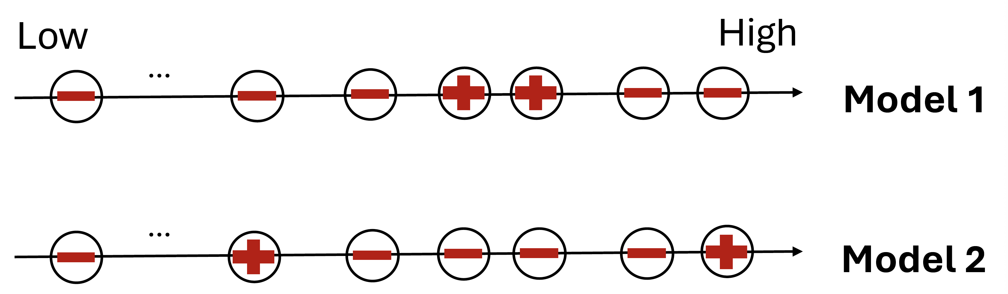
Necessity of Maximizing Partial AUC

In many applications (e.g., medical diagnosis), there are large monetary costs associated with high FPR and low TPR. Hence, a measure of interest is pAUC—the region of the ROC curve corresponding to low FPR and/or high TPR. By an argument analogous to the previous section, maximizing AUC does not necessarily maximize pAUC.

Consider two models on a dataset with two positive and 100 negative molecules (see Figure 2.4). Model 1 ranks two negatives above the two positives, followed by the remaining 98 negatives. Model 2 ranks one positive at the top, then four negatives above the other positive, followed by the remaining 96 negatives. Both models have the same AUC score \(196/200 = 0.98\) but different pAUC scores. Restricting \(\text{FPR} \in [0, 0.02]\), Model 1 has empirical pAUC score of \(\frac{0}{4} = 0\) and Model 2 has empirical pAUC score of \(\frac{2}{4} = 0.5\) according to (\(\ref{eqn:opauc-emp}\)).

Critical: Partial AUC emphasizes the correct order between the top-ranked negatives and/or the bottom-ranked positives.

A Direct Formulation

Using a surrogate of the zero–one loss, OPAUC maximization for learning a parameterized model \(h(\mathbf{w}; \cdot)\) can be formulated as:

\[\begin{align}\label{eqn:epaucd2} \min_{\mathbf{w}} \frac{1}{n_+}\frac{1}{k_2} \sum_{\mathbf{x}_i \in \mathcal{S}_+}\sum_{\mathbf{x}_j \in \mathcal{S}_-^{\downarrow}[1, k_2]} \ell\big(h(\mathbf{w}; \mathbf{x}_j) - h(\mathbf{w}; \mathbf{x}_i)\big). \end{align}\]

Similarly, TPAUC maximization can be formulated as: \[\begin{align}\label{eqn:tpaucd2} \min_{\mathbf{w}} \frac{1}{k_1}\frac{1}{k_2} \sum_{\mathbf{x}_i \in \mathcal{S}_+^{\uparrow}[1, k_1]}\sum_{\mathbf{x}_j \in \mathcal{S}_-^{\downarrow}[1, k_2]} \ell\big(h(\mathbf{w}; \mathbf{x}_j) - h(\mathbf{w}; \mathbf{x}_i)\big), \end{align}\] where \(k_1 = \lfloor n_+ (1-\alpha) \rfloor\), \(k_2 = \lfloor n_- \beta \rfloor\).

Both problems are not standard ERM. The main challenge is that selecting examples in a range (e.g., \(\mathcal{S}_-^{\downarrow}[1,k_2]\), \(\mathcal{S}_+^{\uparrow}[1,k_1]\)) is expensive and non-differentiable. We will explore approaches for optimizing OPAUC and TPAUC in Section 6.3 using advanced compositional optimization techniques.

An Indirect Formulation

When the surrogate loss \(\ell(t)\) is non-decreasing, the top-\(k\) selector of negatives \(\mathcal{S}_-^{\downarrow}[1, k_2]\) can be converted into the top-\(k\) average of pairwise losses, which becomes a CVaR. By connecting CVaR with KL-regularized DRO, an indirect objective for OPAUC maximization is:

\[\begin{align}\label{eqn:epaucd3} \min_{\mathbf{w}} \frac{1}{n_+} \sum_{\mathbf{x}_i \in \mathcal{S}_+} \tau \log\!\left(\sum_{\mathbf{x}_j \in \mathcal{S}_-} \exp\!\left(\frac{\ell\big(h(\mathbf{w}; \mathbf{x}_j) - h(\mathbf{w}; \mathbf{x}_i)\big)}{\tau}\right)\right). \end{align}\]

This is an instance of EXM and will be solved using FCCO techniques. We will present detailed exposition in Section 6.3.

2.3.4 Ranking Losses

Ranking losses are commonly employed in learning to rank.

What is Learning to Rank?
Learning to rank (LTR) is a machine learning problem that aims to learn a ranking model, which can be used to predict the relevance order of a set of items given a query.

Let \(\mathcal{Q}\) denote the query set of size \(N\), and let \(q \in \mathcal{Q}\) represent an individual query. For each query \(q\), let \(\mathcal{S}_q\) be a set of \(N_q\) items (e.g., documents, movies) to be ranked. For each item \(\mathbf{x}_{q,i} \in \mathcal{S}_q\), let \(y_{q,i} \in \mathbb{R}^+\) denote its relevance score, which quantifies the relevance between the query \(q\) and the item \(\mathbf{x}_{q,i}\). Define \(\mathcal{S}^+_q \subseteq \mathcal{S}_q\) as the subset of \(N^+_q\) items relevant to \(q\), i.e., those with non-zero relevance scores. Let \(\mathcal{S} = \{(q, \mathbf{x}_{q,i}) \mid q \in \mathcal{Q}, \mathbf{x}_{q,i} \in \mathcal{S}^+_q\}\) represent the collection of all relevant query-item (Q-I) pairs.

Let \(s(\mathbf{w}; \mathbf{x}, q)\) denote the predicted relevance score for item \(\mathbf{x}\) with respect to query \(q\), parameterized by \(\mathbf{w} \in \mathbb{R}^d\) (e.g., a deep neural network). Define the rank of item \(\mathbf{x}\) within \(\mathcal{S}_q\) as: \[\begin{align*} r(\mathbf{w}; \mathbf{x}, \mathcal{S}_q) = \sum_{\mathbf{x}' \in \mathcal{S}_q} \mathbb{I}(s(\mathbf{w}; \mathbf{x}', q) - s(\mathbf{w}; \mathbf{x}, q) \ge 0), \end{align*}\] where ties are ignored.

NDCG and NDCG Loss

Normalized Discounted Cumulative Gain (NDCG) is a metric commonly used to evaluate the quality of ranking algorithms, especially in information retrieval and recommender systems.

NDCG evaluates how well a model ranks relevant items near the top of a list for a query \(q\). The DCG of a ranked list according to \(\{s(\mathbf{w}; \mathbf{x}, q), \mathbf{x} \in \mathcal{S}_q\}\) is given by: \[ \text{DCG}_q=\sum_{\mathbf{x}\in\mathcal{S}_q}\frac{2^{y_i}-1}{\log_2(1+r(\mathbf{w}; \mathbf{x}, \mathcal{S}_q))} = \sum_{\mathbf{x}\in\mathcal{S}_q^+}\frac{2^{y_i}-1}{\log_2(1+r(\mathbf{w}; \mathbf{x}, \mathcal{S}_q))}. \] Note that the summation is over \(\mathcal{S}^+_q\) rather than \(\mathcal{S}_q\), as only relevant items contribute to the DCG score due to their non-zero relevance.

NDCG normalizes DCG by the ideal DCG denoted by \(Z_q\) of the best possible ranking: \[ \text{NDCG}_q = \frac{\text{DCG}_q}{Z_q}. \] The average NDCG over all queries is given by: \[\begin{align}\label{eqn:NDCG} \text{NDCG:}\quad \frac{1}{N} \sum_{q=1}^N \frac{1}{Z_q} \sum_{\mathbf{x}_{q,i} \in \mathcal{S}^+_q} \frac{2^{y_{q,i}} - 1}{\log_2(r(\mathbf{w}; \mathbf{x}_{q,i}, \mathcal{S}_q) + 1)}, \end{align}\] where \(Z_q\) can be precomputed.

By replacing the indicator function with a surrogate function in Table 2.3, we approximate \(r(\mathbf{w}; \mathbf{x}, \mathcal{S}_q)\) by \[ g(\mathbf{w}; \mathbf{x}, \mathcal{S}_q) = \sum_{\mathbf{x}' \in \mathcal{S}_q} \ell(s(\mathbf{w}; \mathbf{x}', q) - s(\mathbf{w}; \mathbf{x}, q)). \] Then the NDCG loss minimization is defined by \[\begin{align}\label{eqn:NDCG-loss} \min_{\mathbf{w}} \frac{1}{N} \sum_{q=1}^N \frac{1}{Z_q} \sum_{\mathbf{x}_{q,i} \in \mathcal{S}^+_q} \frac{1-2^{y_{q,i}}}{\log_2(g(\mathbf{w}; \mathbf{x}_{q,i}, \mathcal{S}_q) + 1)}, \end{align}\] which is an instance of EXM. We will explore FCCO technique for solving this problem in Section 6.3.

Listwise Cross-Entropy Loss

Analogous to multi-class classification, we can define a listwise cross-entropy loss for ranking. This is based on modeling the probability that a specific item is ranked at the top: \[\begin{align}\label{eqn:dpm-list} P_{\text{top}}(\mathbf{x} \mid q) = \frac{\exp(s(\mathbf{w}; \mathbf{x}, q))}{\sum_{\mathbf{x}_j \in \mathcal{S}_q} \exp(s(\mathbf{w}; \mathbf{x}_j, q))}. \end{align}\] Accordingly, the listwise cross-entropy loss for query \(q\) is defined as: \[\begin{align*} L(\mathbf{w}; q) = \sum_{\mathbf{x}_{q,i} \in \mathcal{S}^+_q} -p_{q,i} \log \left( \frac{\exp(s(\mathbf{w}; \mathbf{x}_{q,i}, q))}{\sum_{\mathbf{x}_j \in \mathcal{S}_q} \exp(s(\mathbf{w}; \mathbf{x}_j, q))} \right), \end{align*}\] where \(p_{q,i}\) denotes the top-one prior probability for item \(\mathbf{x}_{q,i}\), such as \[ p_{q,i} = \frac{\exp(y_{q,i})}{\sum_{\mathbf{x}_{q,i} \in \mathcal{S}_q} \exp(y_{q,i})} \quad \text{or} \quad p_{q,i} = \frac{1}{N_q}. \]

An optimization objective based on the average of listwise cross-entropy losses over all queries leads to the following formulation known as ListNet: \[\begin{align} \label{eqn:listnet} \min_{\mathbf{w}} \quad \frac{1}{N} \sum_{q=1}^N \sum_{\mathbf{x}_{q,i} \in \mathcal{S}^+_q} p_{q,i} \log \left( \sum_{\mathbf{x}_j \in \mathcal{S}_q} \exp(s(\mathbf{w}; \mathbf{x}_j, q) - s(\mathbf{w}; \mathbf{x}_{q,i}, q)) \right). \end{align}\]

This formulation closely resembles equation (\(\ref{eqn:epaucd3}\)) and constitutes a special case of the EXM framework.

2.3.5 Contrastive Losses

Representation learning is a fundamental problem in the era of deep learning and modern AI.

What is Representation Learning?
Representation Learning is a process in machine learning where algorithms extract meaningful patterns from raw data (e.g., images) to create representations that are useful for many downstream tasks, e.g., learning a classifier, data retrieval.

A deep neural network is usually used to extract representation from unstructured raw data. Let \(h(\mathbf{w}; \cdot): \mathcal{X} \rightarrow \mathbb{R}^{d_1}\) denote the representation network that outputs an embedding vector, which is also called the encoder. A meaningful encoder should capture the semantics such that `similar’ data points (positive pairs) are closer to each other and dissimilar data points (negative pairs) are far away from each other in the embedding space.

To conduct the representation learning, the following data is usually constructed. Let \(\mathbf{x}_i\) be an anchor data, and let \(\mathbf{x}^+_i\) denote a positive data of \(\mathbf{x}_i\). Denote by \(\mathcal{S}_i^-\) the set of negative data of \(\mathbf{x}_i\). Let \(s(\mathbf{w}; \mathbf{x}, \mathbf{y})\) denote a similarity score between the two encoded representations. For example, if \(h(\mathbf{w}; \mathbf{x})\) is a normalized vector such that \(\|h(\mathbf{w}; \mathbf{x})\|_2 = 1\), we can use \(s(\mathbf{w}; \mathbf{x}, \mathbf{y}) = h(\mathbf{w}; \mathbf{x})^{\top} h(\mathbf{w}; \mathbf{y})\).

A contrastive loss for each positive pair \((\mathbf{x}_i, \mathbf{x}_i^+)\) is defined by: \[\begin{align}\label{eqn:GCL1} L(\mathbf{w}; \mathbf{x}_i, \mathbf{x}^+_i) = \tau \log\left(\frac{1}{|\mathcal{S}_i^-|}\sum_{\mathbf{y}\in\mathcal{S}_i^-}\exp\left(\frac{s(\mathbf{w}; \mathbf{x}_i, \mathbf{y}) - s(\mathbf{w}; \mathbf{x}_i, \mathbf{x}^+_i)}{\tau}\right)\right). \end{align}\] where \(\tau > 0\) is called the temperature parameter. Given a set of data \(\{(\mathbf{x}_i, \mathbf{x}_i^+, \mathcal{S}_i^-)\}_{i=1}^n\), minimizing a contrastive objective for representation learning is formulated as: \[\begin{equation}\label{eqn:GCL} \begin{aligned} \min_{\mathbf{w}} \;& \frac{1}{n}\sum_{i=1}^n \tau \log\left(\frac{1}{|\mathcal{S}_i^-|}\sum_{\mathbf{y}\in\mathcal{S}_i^-}\exp\left(\frac{s(\mathbf{w}; \mathbf{x}_i, \mathbf{y}) - s(\mathbf{w}; \mathbf{x}_i, \mathbf{x}^+_i)}{\tau}\right)\right). \end{aligned} \end{equation}\] A variant of the contrastive objective is to add a small constant \(\varepsilon > 0\) inside the log: \[\begin{equation}\label{eqn:GCLN} \begin{aligned} \min_{\mathbf{w}} \;& \frac{1}{n}\sum_{i=1}^n \tau \log\left(\varepsilon + \frac{1}{|\mathcal{S}_i^-|}\sum_{\mathbf{y}\in\mathcal{S}_i^-}\exp\left(\frac{s(\mathbf{w}; \mathbf{x}_i, \mathbf{y}) - s(\mathbf{w}; \mathbf{x}_i, \mathbf{x}^+_i)}{\tau}\right)\right). \end{aligned} \end{equation}\]

Traditional supervised representation learning methods construct the positive and negative data using the annotated class labels, such that data in the same class are deemed as positive and data from different classes are considered as negative. However, this requires a large amount of labeled data to learn the encoder, which requires significant human effort in labeling. To address this issue, self-supervised representation learning (SSRL) techniques are employed to fully exploit the vast data readily available on the internet via self-supervision (where \(\mathbf{x}_i, \mathbf{x}_i^+\) are constructed from the data itself) to learn representations that are useful for many downstream tasks, which will be explored more in Section 6.4.

Optimization Challenge

Optimizing the above contrastive objectives is challenging due to the presence of summations both inside and outside the logarithmic function. These losses can be reformulated as special cases of X-risk, where the outer function is \(f(g_i) = \tau \log(g_i)\), and \(g_i\) represents the inner average computed over negative samples associated with each \(\mathbf{x}_i\).